MFA Deployment Analysis

Analysis of the impact of Multi-Factor Authentication (MFA) deployment rate on the likelihood of compromise.

Questions/TODO

• Compare the effectiveness of control coverage compare vs defense-in-depth. How do two partially deployed controls compare to a single widely deployed control?

library(purrr)
library(formattable)
library(ggplot2)
library(plotly)
library(jbplot)

Background

Daniel Woods’ research on the empirical effectiveness of security controls shows that Multi-Factor Authentication (MFA) appears to reduce the likelihood of compromise by as much as 99% for individuals, but implementing MFA doesn’t show the same reduction for organizations, discussed in his paper, Evidence-based cybersecurity policy? A meta-review of security control effectiveness, and his LinkedIn article, What Works in Cybersecurity: MFA.

In particular, research from Microsoft found that MFA reduced the risk of compromise by 99%, and a similar study from Google reported that MFA “prevents 94% of attacks rooted in phishing and 76% of targeted attacks”, while cyber insurance claims data offer conflicting evidence: Marsh (2023) found MFA to be the least effective control, and Marsh (2024) found MFA to be the most effective control.

One aspect of MFA that Daniel discusses (briefly) is the idea that MFA deployment rate may explain the contradictory results, as organizations may have a policy requiring MFA and still have gaps in coverage, allowing credential attacks against accounts that don’t have MFA enabled. This analysis models how coverage affects the effectiveness of MFA using Monte Carlo simulation.

Analysis

To model the impact of deployment rate on attack likelihood, we can simulate an attack against a random user in the organization. If the user doesn’t have MFA, the attack always succeeds (the base rate). If the user has MFA, the attack has a 1% success rate (as I found in my MFA Risk Analysis, a 99% reduction in likelihood leads to dramatically lower expected losses).

Simple Model

We can use the uniform distribution to determine if a user has MFA; if a randomly generated number between 0 and 1 exceeds the MFA deployment rate, \(r\), the user doesn’t have MFA. (This will always be true if \(r = 0\) and never true if \(r = 1\)). For users with MFA, the attack succeeds if a second random uniform number is less than or equal to 0.01.

attack_succeeds <- function(deployment_rate) {
  if (runif(1) > deployment_rate) {
    # no MFA
    TRUE
  } else {
    # has MFA
    runif(1) <= 0.01
  }
}

Attacks with \(r = 0\) should always succeed, and attacks with \(r = 1\) should succeed about 1% of the time:

attack_succeeds(0)

[1] TRUE

attack_succeeds(1)

[1] FALSE

sum(replicate(10000, attack_succeeds(1))) # should be close to 100

[1] 107

Instead of using replicate() for repeated trials, we can take advantage of R vectors, which are faster (allowing more trials):

attack_success_rate <- function(deployment_rate, runs = 1e5) {
  has_mfa <- runif(runs) <= deployment_rate
  attack_fails <- runif(runs) <= (has_mfa * 0.99)
  sum(!attack_fails) / runs
}

We should expect an attack success rate of 100% with 0% deployment and approximately 1% with 100% deployment:

attack_success_rate(0)

[1] 1

attack_success_rate(1)

[1] 0.01001

Effect of Deployment Rate

Model the effects of deployment rate on attack success using purrr:map_dbl():

deployment <- (1:100) / 100
success_rate <- map_dbl(deployment, attack_success_rate)
deployment_success <- data.frame(deployment, success_rate)

Plot the results:

deployment_success |>
  ggplot(aes(deployment, success_rate)) +
  geom_point() +
  scale_x_continuous(labels = scales::label_percent()) +
  scale_y_continuous(labels = scales::label_percent()) +
  labs(title = "Effects of MFA deployment rate on attacker success rate") +
  labs(x = "MFA deployment rate", y = "Attacker success rate") +
  theme_quo()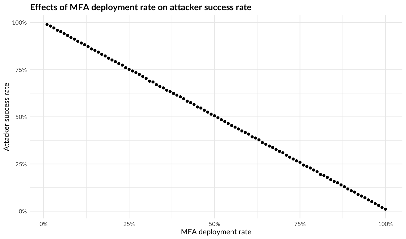

Economic Impact of Deployment Rate

Perhaps unsurprisingly in retrospect, there is a clear linear relationship between deployment rate and attacker success rate. However, as the earlier MFA Analysis shows, expected losses drop dramatically as the likelihood of an attack approaches 0. A plot from that analysis compares baseline risk (no treatment) against a pessimistic estimate of MFA attack success rate reduction (76%) and an optimistic reduction (99%):

load("objects/mfa-exports.RData")
risk_le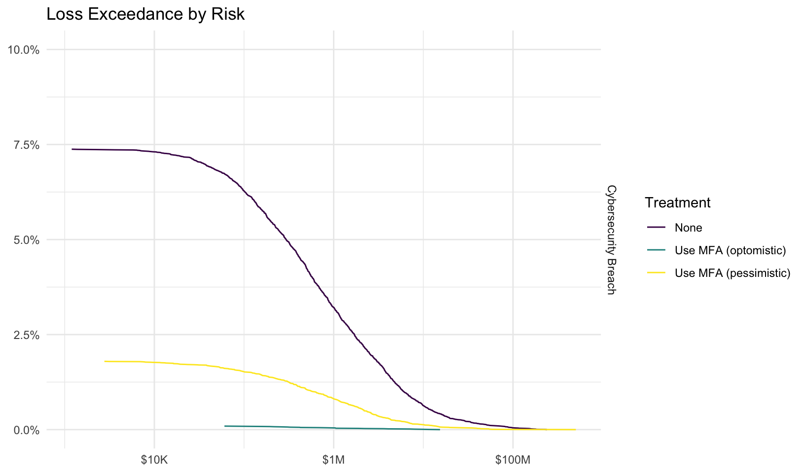

ggsave("rendered/mfa-loss-exceedance.png", width = 16 * 0.6, height = 9 * 0.6, create.dir = TRUE)

Interactive plot:

ggplotly(risk_le + guides(color = "none"))

In the base case, the firm has a 3.2% chance of a loss exceeding $1M (about once every 30 years), which drops to 0.80% with a 76% lower attack success rate (once every 125 years), and 0.04% with a 99% reduction (once every 2500 years).

Successful Attack Frequency

Instead of expressing attacker success as a percentage (rate), we can instead express it in terms of frequency; about how many attacks does it take before an attacker is successful?

frequency_plot <- deployment_success |>
  mutate(
    deployment = percent(deployment, 0), success_rate = percent(success_rate),
    frequency = 1 / success_rate
  ) |>
  ggplot(aes(deployment, frequency, text = paste0("success_rate: ", success_rate))) +
  geom_point() +
  scale_x_continuous(labels = scales::label_percent()) +
  labs(title = "Effects of MFA deployment rate on frequency of succesful attacks") +
  labs(x = "MFA deployment rate", y = "Frequency (attacker succeeds every n tries)") +
  theme_quo()

ggplotly(frequency_plot)

ggsave("rendered/mfa-deployment-rate.png", width = 16 * 0.6, height = 9 * 0.6)

This plot more clearly explains the effect of deployment rate on how often attacks succeed; at 50% deployment, the attack succeeds about every 2 tries. At a deployment rate of 91%, the attack succeeds every 10 tries. A 100% deployment rate (every 100 tries) is about twice as effective as a 99% deployment rate (every 50 tries) - this is true on both plots, but easier to see with the second.

Discussion

While this analysis could have been easily accomplished with probability math, I have found that using models and Monte Carlo simulations helps me understand the results.