MFA Risk Analysis Report
Example quantrr risk analysis of multi-factor authentication (MFA) using real data! Originally used for the plot in my Aug 28 LinkedIn Post.
Environment Statement
Background assumptions:
Professional services firm with $5M in annual revenue. A loss of 1% ($50K) is considered material.
Supplementary Material from the Cyentia IRIS 2025 Report found that the likelihood of at least 1 incident in the next year is 7.48% for firms with less than $10M in revenue.
Figure A3 from the main IRIS 2025 Report shows that the median loss for the Professional sector is $736K and the 95th percentile is $17M. From this we use trial and error to calculate the 50% (median) loss at $31,900.
According to a preprint study, implementing MFA reduces the likelihood of compromise by 99%. An older study found that MFA reduced the likelihood of targeted attacks by 76%.
Note: the research on MFA looked at individuals, and other research on organizations found a lower reduction. For this analysis, we assume the individual risk reduction is achievable with a thorough and complete MFA implementation (fully implemented everywhere).
Import
Import and validate data from Excel.
We use the IRIA 2025 data for the 5th, median, and 95th percentile of impact in all treatments, and adjust the frequency by 99% in the optimistic case and 76% in the pessimistic case.
Code
risks <- read_xlsx(report_file, sheet = "Risks") |>
  clean_names()

validate_risks <- local({
  validate_rules <- validator(
    risk_char = is.character(risk),
    risk_not_na = !is.na(risk),
    risk_not_blank = nzchar(risk, keep_na = TRUE),
    desc_char = is.character(description),
    desc_not_na = !is.na(description),
    desc_not_blank = nzchar(risk, keep_na = TRUE)
  )
  confront(risks, validate_rules)
})

check_validation(validate_risks, sheet = "Risks")

treatments <- read_xlsx(report_file, sheet = "Treatments") |>
  clean_names()

validate_treatments <- local({
  validate_rules <- validator(
    treatment_char = is.character(treatment),
    treatment_not_na = !is.na(treatment),
    treatment_not_blank = nzchar(treatment, keep_na = TRUE),
    desc_char = is.character(description),
    desc_not_na = !is.na(description),
    desc_not_blank = nzchar(treatment, keep_na = TRUE)
  )
  confront(treatments, validate_rules)
})

check_validation(validate_treatments, sheet = "Treatments")

estimates <- read_xlsx(report_file, sheet = "Estimates") |>
  clean_names() |>
  rename(
    lambda = frequency_per_yer, p50 = most_likely, p95 = high_95_percent, p05 = low_5_percent
  )

validate_estimates <- local({
  validate_rules <- validator(
    risk_not_na = !is.na(risk),
    risk_match = risk %in% risks$risk,
    expert_char = is.character(expert),
    expert_not_na = !is.na(expert),
    expert_not_blank = nzchar(expert, keep_na = TRUE),
    lambda_num = is.numeric(lambda),
    lambda_pos = lambda > 0,
    p50_num = is.numeric(p50),
    p50_pos = p50 > 0,
    p95_num = is.numeric(p95),
    p95_pos = p95 > 0,
    p05_num = is.numeric(p05),
    p05_pos = p05 > 0
  )
  confront(estimates, validate_rules)
})

check_validation(validate_estimates, sheet = "Estimates")
Risks
Risk descriptions:
Code
formattable(risks, align = "l")| risk | description |
|---|---|
| Cybersecurity Breach | Risk of a cybersecurity breach |
Treatment descriptions:
Code
formattable(treatments, align = "l")| treatment | description |
|---|---|
| None | Current system as it is today |
| Use MFA | Fully implement MFA for all accounts |
Forecast
Forecast risk using Monte Carlo simulation. The average events, losses, ‘typical’ losses (geometric mean), and percentage of years with no losses for each risk and treatment are summarized below:
Code
consensus <- estimates |>
  group_by(treatment, risk) |>
  summarize(across(lambda:p05, ~ mean(.x, na.rm = TRUE)), .groups = "drop")

consensus_params <- consensus |>
  mutate(as_tibble(lnorm_param(p50 = .data$p50, p95 = .data$p95, p05 = .data$p05)))

forecast <- consensus_params |>
  select(c("risk", "lambda", "meanlog", "sdlog", "treatment")) |>
  pmap(calc_risk) |>
  list_rbind()

forecast |>
  group_by(treatment, risk) |>
  mutate(no_losses = events == 0) |>
  summarize(
    avg_events = mean(events), avg_losses = mean(losses), typ_losses = gmean(losses),
    no_losses = mean(no_losses), .groups = "drop"
  ) |>
  mutate(
    across(avg_losses:typ_losses, ~ currency(.x, digits = 0L)),
    no_losses = percent(no_losses)
  ) |>
formattable(align = "l")| treatment | risk | avg_events | avg_losses | typ_losses | no_losses |
|---|---|---|---|---|---|
| None | Cybersecurity Breach | 0.07292 | $337,423 | $738,129 | 92.99% |
| Use MFA (optomistic) | Cybersecurity Breach | 0.00072 | $1,282 | $477,569 | 99.93% |
| Use MFA (pessimistic) | Cybersecurity Breach | 0.01900 | $103,114 | $832,745 | 98.12% |
Losses
Base losses (with no risk treatment) by risk:
Code
forecast |>
  filter(tolower(treatment) == "none") |>
  # remove zero losses to plot using log10 scale
  filter(losses > 0) |>
  ggplot(aes(losses)) +
  facet_grid(vars(risk)) +
  geom_histogram(color = "black", fill = "white", bins = 100) +
  scale_x_log10(labels = scales::label_currency(scale_cut = scales::cut_short_scale())) +
  labs(x = NULL, y = NULL, title = "Base Losses by Risk") +
  theme_minimal()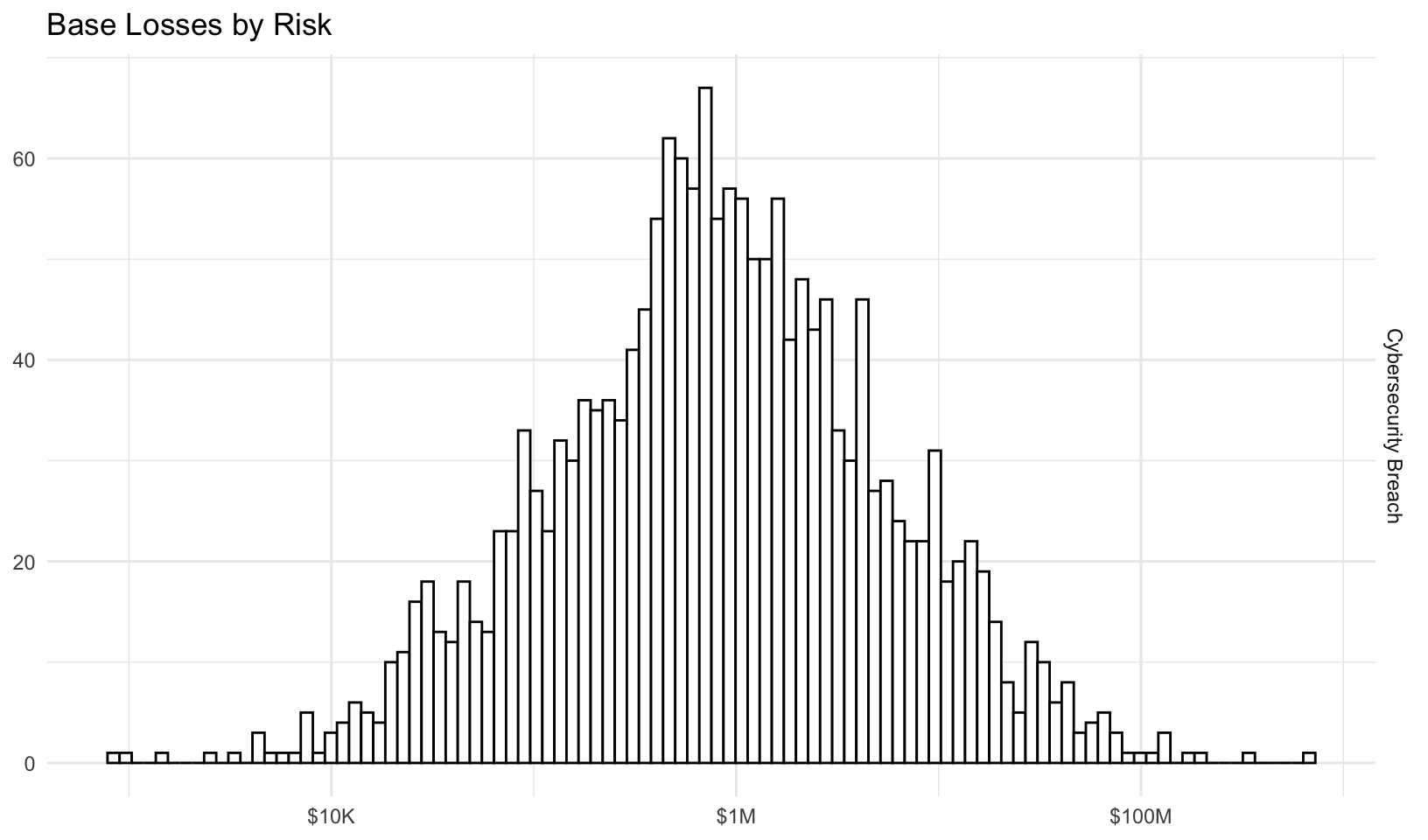
Combined losses by treatment:
Code
forecast |>
  group_by(treatment, year) |>
  summarize(total_losses = sum(losses), .groups = "drop_last") |>
  # remove zero losses to plot using log10 scale
  filter(total_losses > 0) |>
  ggplot(aes(total_losses)) +
  facet_grid(vars(treatment)) +
  geom_histogram(color = "black", fill = "white", bins = 100) +
  scale_x_log10(labels = scales::label_currency(scale_cut = scales::cut_short_scale())) +
  labs(x = NULL, y = NULL, title = "Combined Losses by Treatment") +
  theme_minimal()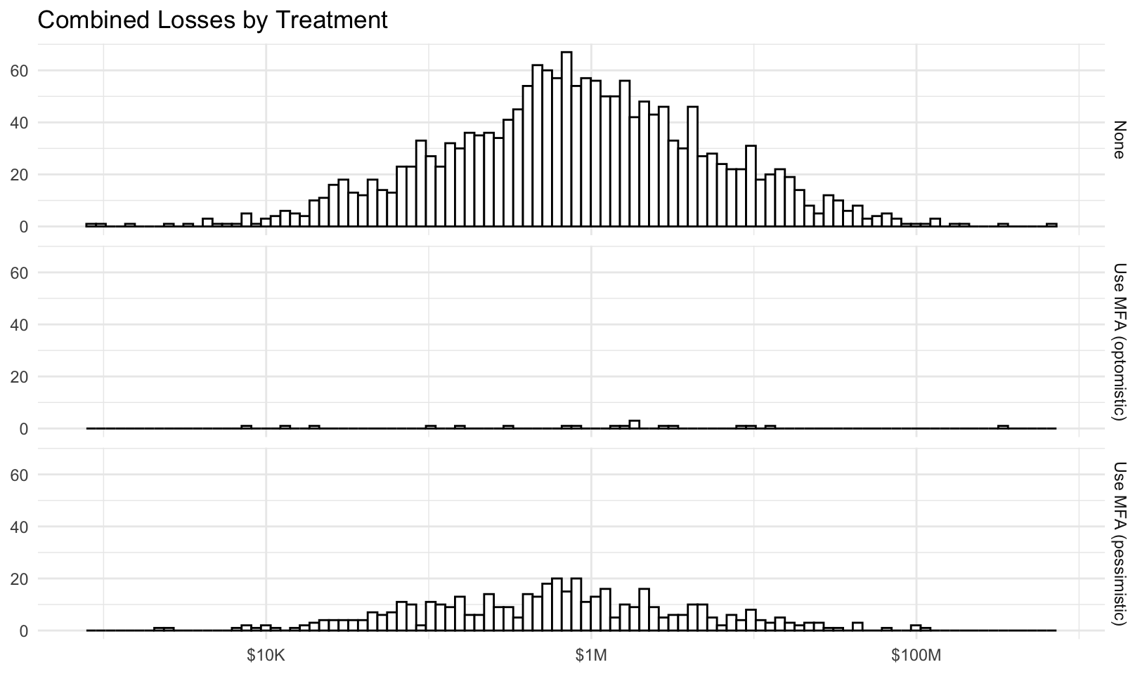
Loss Exceedance Curves
Plot loss exceedance curves for all risks and combined risk, with risk treatments.
By Risk
Plot loss exceedance curves for each risk:
Code
risk_le <- forecast |>
  group_by(risk, treatment) |>
  mutate(probability = 1 - percent_rank(losses)) |>
  filter(losses > 0) |>
  ungroup() |>
  mutate(losses = currency(losses, digits = 0), probability = percent(probability)) |>
  ggplot(aes(losses, probability, color = treatment)) +
  facet_grid(vars(risk)) +
  geom_line() +
  scale_y_continuous(labels = scales::label_percent(), limits = c(0, 0.1)) +
  scale_x_log10(labels = scales::label_currency(scale_cut = scales::cut_short_scale())) +
  labs(x = NULL, y = NULL, color = "Treatment", title = "Loss Exceedance by Risk") +
  scale_color_viridis_d() +
  theme_minimal()

risk_le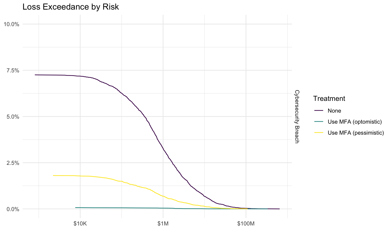
Interactive plot:
Combined Risk
Plot loss exceedance curve for combined risk:
Code
combined_le <- forecast |>
  group_by(treatment, year) |>
  summarize(total_losses = sum(losses), .groups = "drop_last") |>
  mutate(probability = 1 - percent_rank(total_losses)) |>
  filter(total_losses > 0) |>
  ungroup() |>
  mutate(total_losses = currency(total_losses, digits = 0), probability = percent(probability)) |>
  ggplot(aes(total_losses, probability, color = treatment)) +
  geom_line() +
  scale_y_continuous(labels = scales::label_percent(), limits = c(0, 0.1)) +
  scale_x_log10(labels = scales::label_currency(scale_cut = scales::cut_short_scale())) +
  labs(x = NULL, y = NULL, color = "Treatment", title = "Combined Loss Exceedance") +
  scale_color_viridis_d() +
  theme_minimal()

combined_le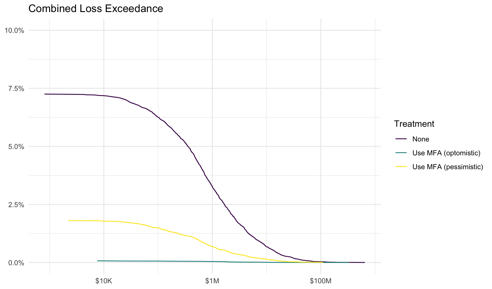
Interactive plot:
Appendix
Additional details on the risk quantification analysis.
Validation
Data validation results for Risks tab:
Code
plot(validate_risks)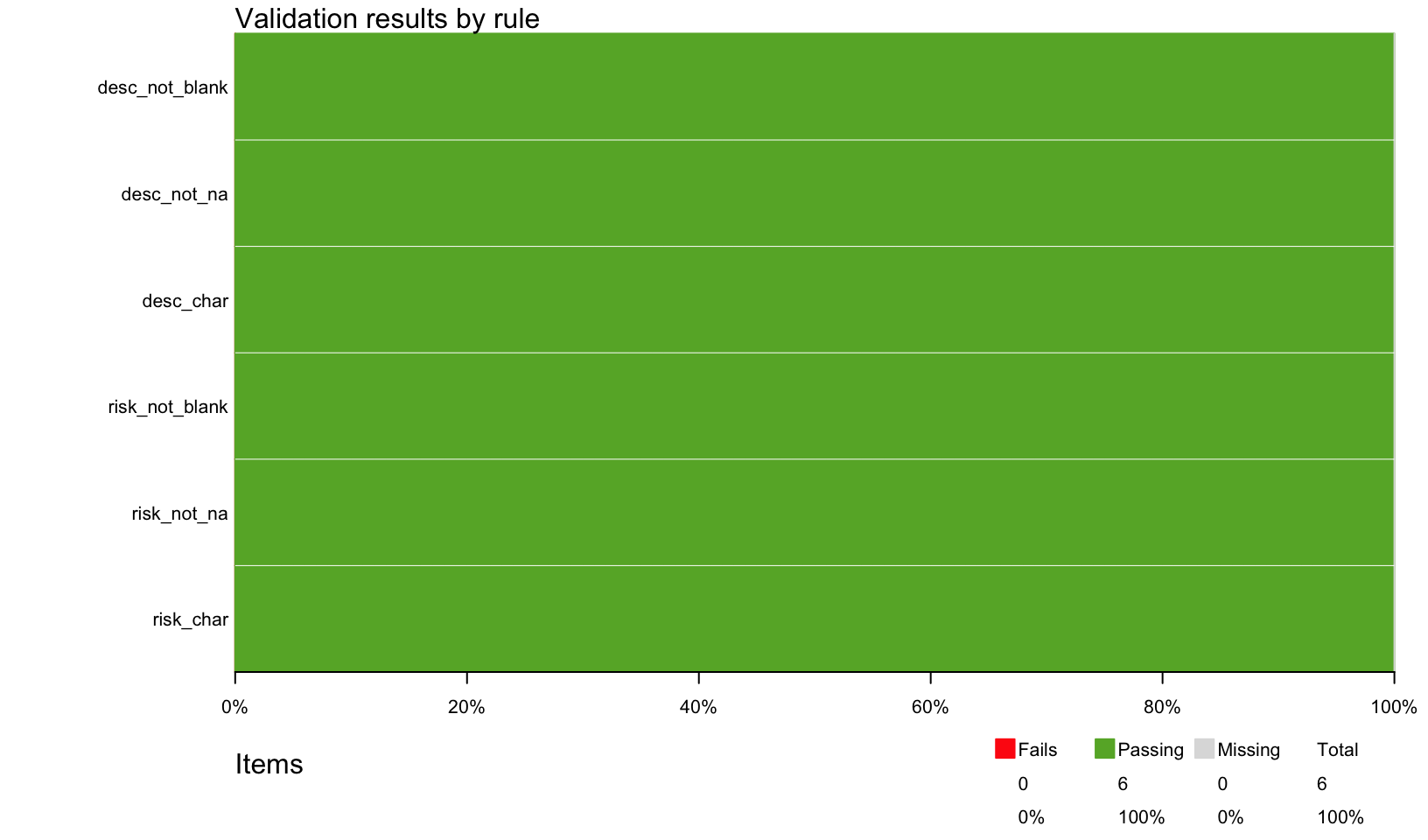
Data validation results for Treatments tab:
Code
plot(validate_treatments)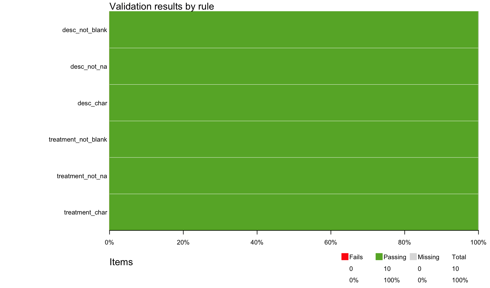
Data validation results for Estimates tab:
Code
plot(validate_estimates)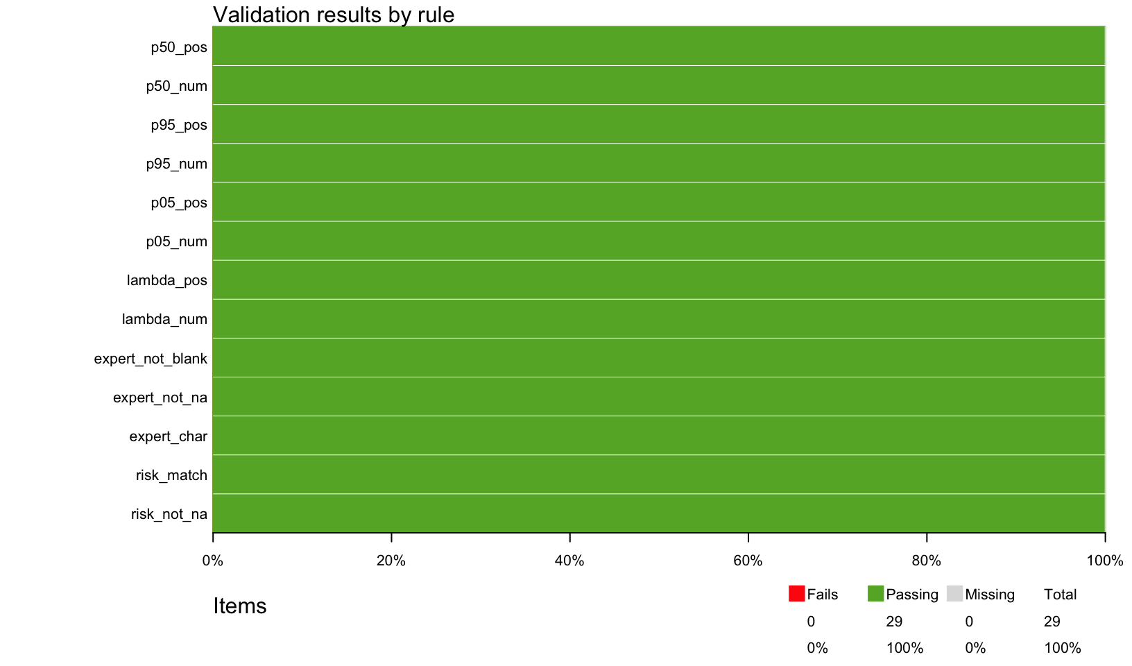
Estimates
All risk estimates:
Code
estimates |>
  mutate(across(p50:p05, ~ currency(.x, digits = 0L))) |>
formattable(align = "l")| treatment | risk | expert | lambda | p50 | p95 | p05 |
|---|---|---|---|---|---|---|
| None | Cybersecurity Breach | IRIS | 0.074800 | $736,000 | $17,000,000 | $31,900 |
| Use MFA (optomistic) | Cybersecurity Breach | Paper | 0.000748 | $736,000 | $17,000,000 | $31,900 |
| Use MFA (pessimistic) | Cybersecurity Breach | Paper | 0.017952 | $736,000 | $17,000,000 | $31,900 |
Consensus Estimate
Using a simple average of all experts that provided an estimate (not blank/NA), this gives us a consensus estimate for the three risks of:
Code
consensus |>
  mutate(across(p50:p05, ~ currency(.x, digits = 0L))) |>
formattable(align = "l")| treatment | risk | lambda | p50 | p95 | p05 |
|---|---|---|---|---|---|
| None | Cybersecurity Breach | 0.074800 | $736,000 | $17,000,000 | $31,900 |
| Use MFA (optomistic) | Cybersecurity Breach | 0.000748 | $736,000 | $17,000,000 | $31,900 |
| Use MFA (pessimistic) | Cybersecurity Breach | 0.017952 | $736,000 | $17,000,000 | $31,900 |
The consensus estimates result in the following parameters for log-normal loss magnitude. When both p05 and p95 are provided, the p50 estimate is used to calculate the percentage difference from the actual median (mdiff), a measure of estimate accuracy (otherwise mdiff is NA):
Code
consensus_params |>
  mutate(across(p05:p50, ~ currency(.x, digits = 0L)), mdiff = percent(mdiff)) |>
formattable(align = "l")| treatment | risk | lambda | p50 | p95 | p05 | meanlog | sdlog | mdiff |
|---|---|---|---|---|---|---|---|---|
| None | Cybersecurity Breach | 0.074800 | $736,000 | $17,000,000 | $31,900 | 13.50954 | 1.908487 | -0.06% |
| Use MFA (optomistic) | Cybersecurity Breach | 0.000748 | $736,000 | $17,000,000 | $31,900 | 13.50954 | 1.908487 | -0.06% |
| Use MFA (pessimistic) | Cybersecurity Breach | 0.017952 | $736,000 | $17,000,000 | $31,900 | 13.50954 | 1.908487 | -0.06% |
Forecast Summary
A summary() of the forecast results.
Code
summary(forecast) year risk treatment events
Min. : 1 Length:75000 Length:75000 Min. :0.00000
1st Qu.: 6251 Class :character Class :character 1st Qu.:0.00000
Median :12500 Mode :character Mode :character Median :0.00000
Mean :12500 Mean :0.03088
3rd Qu.:18750 3rd Qu.:0.00000
Max. :25000 Max. :3.00000
losses
Min. : 0
1st Qu.: 0
Median : 0
Mean : 147273
3rd Qu.: 0
Max. :363833184