library(poilog)
library(tibble)
library(dplyr)
library(quantrr)
library(formattable)
library(ggplot2)
library(plotly)
library(jbplot)Risk Value Analysis
risk quantification
An exploration of the value of cybersecurity risk reduction.
Questions/TODO
Background
What is the value of a cybersecurity program? Put another way, how much should an organization pay to reduce the likelihood of a breach or the expected impact? In this analysis, we compare two firms, one with typical breach rate and impact, and a second that makes investments to reduce their risk. Using Monte Carlo simulation, we can calculate the value of this risk reduction.
For the analysis, we use a 10 year horizon to fit with the typical executive tenure of 5-10 years. (A 2023 study found that CISOs at Fortune 500 companies had served an average of 8.3 years at the company and 4.5 years as CISO)
Baseline Risk
We can model baseline risk for a typical firm using quantrr and data from the Cyentia 2022 Information Risk Insights Study (IRIS).
The 2022 IRIS found that the upper bound likelihood of a breach in the next year fit a Poisson log-normal distribution with a mean (\(\mu\)) of -2.284585 and and standard deviation (\(\sigma\)) of 0.8690759.
As was done in the breach rate analysis, we can use trial and error to find a reasonable value of \(\lambda\) for a Poisson distribution that approximates these results without increasing the number of breaches (it underestimates the number of multiple breaches but replicates the number of single breaches):
runs <- 1e6
lambda <- 0.138
breaches_poilog <- rpoilog(runs, mu = -2.284585, sig = 0.8690759, keep0 = TRUE)
breaches_pois <- rpois(runs, lambda = lambda)
breach_table <- function(breaches) {
years <- length(breaches)
tibble(
"One or more" = sum(breaches >= 1) / years,
"Two or more" = sum(breaches >= 2) / years,
"Three or more" = sum(breaches >= 3) / years
)
}
bind_rows(breach_table(breaches_poilog), breach_table(breaches_pois))# A tibble: 2 × 3
`One or more` `Two or more` `Three or more`
<dbl> <dbl> <dbl>
1 0.129 0.0165 0.00249
2 0.128 0.00857 0.000396A Poisson distribution with a \(\lambda\) of 0.138 approximates the Poisson log-normal model from the Cyentia IRIS report.
meanlog <- 12.55949
sdlog <- 3.068723For the impact, we can use the log-normal loss model from IRIS, with a mean (\(\mu\)) of 12.55949 and standard deviation(\(\sigma\)) of 3.068723.
Using the baseline parameters, we can simulate security events and losses over the next 10 years:
calc_risk("baseline", lambda, meanlog, sdlog, runs = 10) |>
mutate(losses = currency(losses, digits = 0))# A tibble: 10 × 5
year risk treatment events losses
<int> <chr> <chr> <int> <formttbl>
1 1 baseline none 0 $0
2 2 baseline none 0 $0
3 3 baseline none 0 $0
4 4 baseline none 0 $0
5 5 baseline none 0 $0
6 6 baseline none 0 $0
7 7 baseline none 0 $0
8 8 baseline none 0 $0
9 9 baseline none 0 $0
10 10 baseline none 0 $0 Net Present Value
We can calculate the (negative) net present value of the baseline security risk over the next ten years by discounting future years. A discount rate of 5% is reasonable, and we use the formula \(\mathrm{NPV} = \large \frac{R_t}{(1+i)^t}\), treating year 1 as \(t = 0\):
rate <- 0.05
baseline_value <- calc_risk("baseline", lambda, meanlog, sdlog, runs = 10) |>
mutate(
losses = currency(losses, digits = 0), discount = (1 + rate)^(year - 1),
value = losses / discount
)
baseline_value# A tibble: 10 × 7
year risk treatment events losses discount value
<int> <chr> <chr> <int> <formttbl> <dbl> <formttbl>
1 1 baseline none 0 $0 1 $0
2 2 baseline none 0 $0 1.05 $0
3 3 baseline none 0 $0 1.10 $0
4 4 baseline none 1 $2,521,472 1.16 $2,178,143
5 5 baseline none 0 $0 1.22 $0
6 6 baseline none 0 $0 1.28 $0
7 7 baseline none 0 $0 1.34 $0
8 8 baseline none 0 $0 1.41 $0
9 9 baseline none 2 $6,536,378 1.48 $4,424,078
10 10 baseline none 0 $0 1.55 $0 baseline_value |>
group_by(risk) |>
summarize(npv = sum(value))# A tibble: 1 × 2
risk npv
<chr> <formttbl>
1 baseline $6,602,220The baseline value is highly variable depending on how many breaches occur over the 10-year period. We can forecast this range by running the 10-year simulation 100,000 times:
baseline_forecast <- calc_risk("baseline", lambda, meanlog, sdlog, runs = 100000 * 10) |>
mutate(
sim = ceiling(year / 10),
year = year %% 10,
year = if_else(year == 0, 10, year),
discount = (1 + rate)^(year - 1),
value = losses / discount
) |>
group_by(sim) |>
summarize(npv = sum(value))
baseline_forecast |>
filter(npv != 0) |>
ggplot(aes(npv)) +
geom_hist_bw(bins = 100) +
scale_x_log10(labels = scales::label_currency(scale_cut = scales::cut_short_scale())) +
labs(x = NULL, y = NULL) +
theme_quo()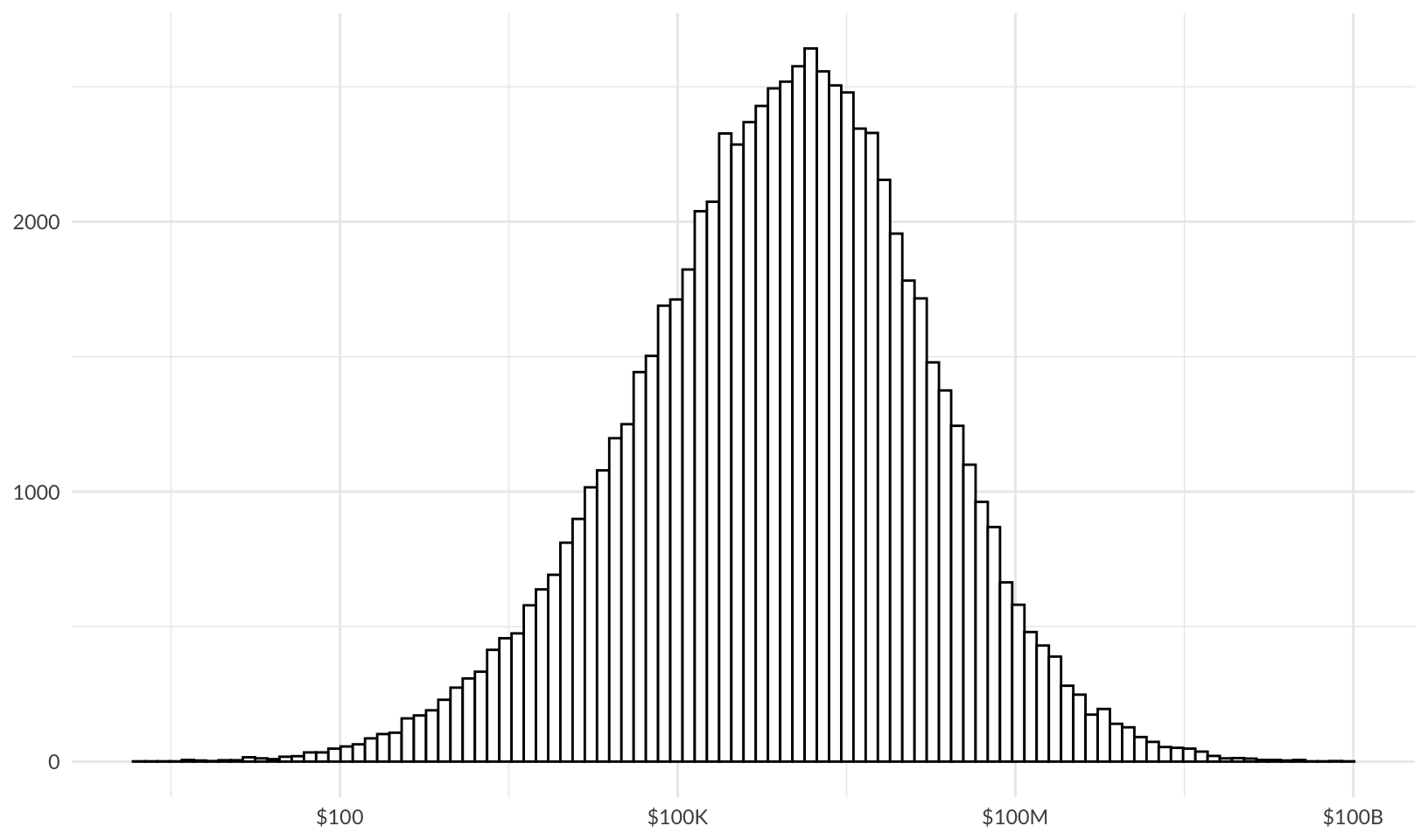
That’s a broad range, from $100 or less to $10B or more, with the most common non-zero value around $1M. But how many runs have no loss?
baseline_forecast |>
mutate(no_loss = (npv == 0)) |>
count(no_loss)# A tibble: 2 × 2
no_loss n
<lgl> <int>
1 FALSE 74639
2 TRUE 25361About 25% of the time, there is no loss over the 10 year period.
Security NPV
What is the NPV of a hypothetical security investment? The key ways we can reduce risk are by lowering the likelihood, by lowering the impact, or both.
Reduce Likelihood
Let’s first look at an investment that reduces the breach rate by half:
likelihood_forecast <- calc_risk("likelihood", lambda / 2, meanlog, sdlog, runs = 100000 * 10) |>
mutate(
sim = ceiling(year / 10),
year = year %% 10,
year = if_else(year == 0, 10, year),
discount = (1 + rate)^(year - 1),
value = losses / discount
) |>
group_by(sim) |>
summarize(npv = sum(value))To measure the value of this investment, we calculate the difference between the baseline risk and the risk after reducing the likelihood:
likelihood_return <-
full_join(baseline_forecast, likelihood_forecast, by = "sim", suffix = c("_base", "_reduced")) |>
mutate(return = npv_base - npv_reduced)
head(likelihood_return, 10)# A tibble: 10 × 4
sim npv_base npv_reduced return
<dbl> <dbl> <dbl> <dbl>
1 1 423910. 20095468. -19671558.
2 2 5674768. 0 5674768.
3 3 0 0 0
4 4 7507846. 9064. 7498782.
5 5 426174. 32469. 393705.
6 6 827229. 0 827229.
7 7 0 1108950. -1108950.
8 8 5621042. 0 5621042.
9 9 93934. 0 93934.
10 10 20384828. 775702. 19609126.summary(likelihood_return) sim npv_base npv_reduced return
Min. : 1 Min. :0.000e+00 Min. :0.000e+00 Min. :-2.318e+11
1st Qu.: 25001 1st Qu.:0.000e+00 1st Qu.:0.000e+00 1st Qu.:-4.849e+04
Median : 50000 Median :2.509e+05 Median :0.000e+00 Median : 5.505e+04
Mean : 50000 Mean :3.151e+07 Mean :2.054e+07 Mean : 1.096e+07
3rd Qu.: 75000 3rd Qu.:3.122e+06 3rd Qu.:4.816e+05 3rd Qu.: 2.350e+06
Max. :100000 Max. :2.259e+11 Max. :2.318e+11 Max. : 2.259e+11 The NPV of the risk reduction (return) is highly variable, and sometimes negative, because even though we’ve reduced the overall risk, in a given 10 year period we might be unlucky and experience a larger breach than in the baseline scenario. Since we can’t plot negative numbers using a log scale, we can examine the data using the cumulative distribution function (CDF). We limit the x-axis to zoom in to the 1% to 99% quantiles:
(likelihood_return |>
ggplot(aes(return)) +
stat_ecdf() +
coord_cartesian(
xlim = c(quantile(likelihood_return$return, 0.01), quantile(likelihood_return$return, 0.99))
) +
labs(x = NULL, y = NULL) +
theme_minimal()) |>
ggplotly()Reviewing the data:
- About 40% of the time, our security investment has a negative or zero return
- About 15% of the time, the security investment has a negative return of over $1M
- About 60% of the time, the security investment has a positive return
- About 32% of the time, the security investment has a positive return of over $1M
- The median (50%) return is about $60,000
Reduce Impact
Now let’s look at an investment that reduces the breach impact by half:
impact_forecast <- calc_risk("impact", lambda, meanlog - log(2), sdlog, runs = 100000 * 10) |>
mutate(
sim = ceiling(year / 10),
year = year %% 10,
year = if_else(year == 0, 10, year),
discount = (1 + rate)^(year - 1),
value = losses / discount
) |>
group_by(sim) |>
summarize(npv = sum(value))To measure the value of this investment, we calculate the difference between the baseline risk and the risk after reducing the likelihood:
impact_return <-
full_join(baseline_forecast, impact_forecast, by = "sim", suffix = c("_base", "_reduced")) |>
mutate(return = npv_base - npv_reduced)
summary(impact_return) sim npv_base npv_reduced return
Min. : 1 Min. :0.000e+00 Min. :0.000e+00 Min. :-1.846e+11
1st Qu.: 25001 1st Qu.:0.000e+00 1st Qu.:0.000e+00 1st Qu.:-6.459e+05
Median : 50000 Median :2.509e+05 Median :1.272e+05 Median : 1.151e+03
Mean : 50000 Mean :3.151e+07 Mean :1.935e+07 Mean : 1.215e+07
3rd Qu.: 75000 3rd Qu.:3.122e+06 3rd Qu.:1.578e+06 3rd Qu.: 2.019e+06
Max. :100000 Max. :2.259e+11 Max. :1.846e+11 Max. : 2.259e+11 Again, the NPV of the risk reduction (return) is highly variable. We again examine the data using the cumulative distribution function (CDF), limiting the x-axis:
(impact_return |>
ggplot(aes(return)) +
stat_ecdf() +
coord_cartesian(
xlim = c(quantile(impact_return$return, 0.01), quantile(impact_return$return, 0.99))
) +
labs(x = NULL, y = NULL) +
theme_minimal()) |>
ggplotly()Reviewing the data:
- About 50% of the time, our security investment has a negative or zero return
- About 22% of the time, the security investment has a negative return of over $1M
- About 50% of the time, the security investment has a positive return
- About 30% of the time, the security investment has a positive return of over $1M
- The median (50%) return is about $1,000
Analysis
What can we learn from these simulations? While a security investment is more likely than not to have a positive return, it’s not a particularly good bet. Over a reasonable planning horizon for a typical executive, it’s hard for an investment with a variable return to compete with investments that have a clear expected positive return. As a CISO, it’s a reasonable choice to simply maintain the status quo of the baseline risk, as there’s a good chance that there will be no breaches (25%) or breaches with lower impact:
baseline_forecast |>
pull(npv) |>
quantile(0.5) |>
currency() 50%
$250,867.66 Put another way, the analysis helps explain why firms don’t invest more in security: the firms’ managers are better off prioritizing non-security investments, and (potentially) blaming the CISO when breaches do occur, especially if they have limited their risk by purchasing cybersecurity insurance. A rational manager will minimize investments in security unless mandated by insurance or if increasing security spend is more than offset by reductions in premiums.
For the most part, this is what we often see in practice: security leaders struggling to get funding to improve security beyond what is minimally expected by external stakeholders (clients, regulators, and insurers). However, we also see certain larger organizations invest more in security, like large banks and other financial institutions, why is this? Work done by VivoSecurity in forecasting data breaches suggests an answer. Vivo found a positive correlation between the size of an organization and the likelihood of a security breach (which has also been identified by others, like Cyentia), and also found a negative correlation with the number of CISAs and CISSPs on staff. The correlation was stronger when looking at the effect on larger breaches.
I believe what this correlation shows is that the overall level of security investment at a firm, as measured by the headcount of certified professionals, has a big impact on reducing the likelihood of the largest breaches of $1M or higher. From the same presentation, the Vivo model predicts fairly frequent small breaches (under $100K) at three of the largest Canadian banks, but large breaches are very rare (under 1% for breaches in the $1M-$10M range). The high level of investment at older banks may also be partly explained by the fact that their security programs predate commercial cyber insurance. This insight is not captured in the simple model presented here.
Implications
What are the implications for security? At a macro level, I think this is an argument for regulation, either government regulation or private regulation through the insurance market. Historically we’ve seen both happen in fire safety: government regulation through building codes has reduced the risk of fire and loss of life over time, and insurance-driven regulations - UL, founded as Underwriters Laboratories, was initially funded by fire insurance companies.
At the firm level, I think this means that security leaders shouldn’t present security as an investment. As with safety, I think the main argument for better security is a moral or emotional case: we care about security because we care about our customers, partners, and other stakeholders. Also, people are typically loss-averse, so expressing security risk in those terms will better connect with decision makers. Using Tail value at risk or Loss Exceedance Curves express loss in this way - “There’s a 5% chance of cybersecurity losses exceeding $780,000 and a 1% chance of losses exceeding $25,000,000 over the next year.” I also think it means security leaders should be mindful of how they spend their limited funds, by maximizing investments in what works.
A Counterexample
After completing my initial analysis, I remembered a counterexample: in one of his last presentations, Marcus Ranum described the layered security controls he helped put in place at an entertainment company that “didn’t want to be next” after the 2014 Sony attack. Marcus worked with their security team to implement a combination of encrypted drives, next-gen firewalls, and whitelisting products to dramatically reduce malware attacks against corporate endpoints. One of the surprising outcomes was that the investment in installing the new controls was more than offset by a reduction in operational costs responding to malware.
So it’s clear that security can be a good investment, but why? The conclusions in the initial analysis rely on the fact that security breaches are relatively infrequent, which was not the case for malware response at the company Marcus worked with. Additionally, these low-level infections aren’t likely to make their way into the public dataset used by the Cyentia IRIS report.
High-Frequency Incidents
We can repeat the analysis looking at malware with a hypothetical 50% reduction in frequency. In a large organization, we might expect to respond to clean up a malware infection once a week (\(\lambda = 52\)) with 90% of incidents costing between $200 and $2000 to clean up, with a typical response cost of $600. To simplify the analysis, we just look at the cost of the next year:
lnorm_param(p05 = 200, p95 = 2000, p50 = 600)$meanlog
[1] 6.44961
$sdlog
[1] 0.6999362
$mdiff
[1] -0.0513167baseline_malware <- calc_risk("baseline malware", lambda = 52, meanlog = 6.44961, sdlog = 0.6999362)
baseline_malware |>
ggplot(aes(losses)) +
geom_hist_bw(bins = 100) +
scale_x_continuous(labels = scales::label_currency(scale_cut = scales::cut_short_scale())) +
labs(x = NULL, y = NULL) +
theme_quo()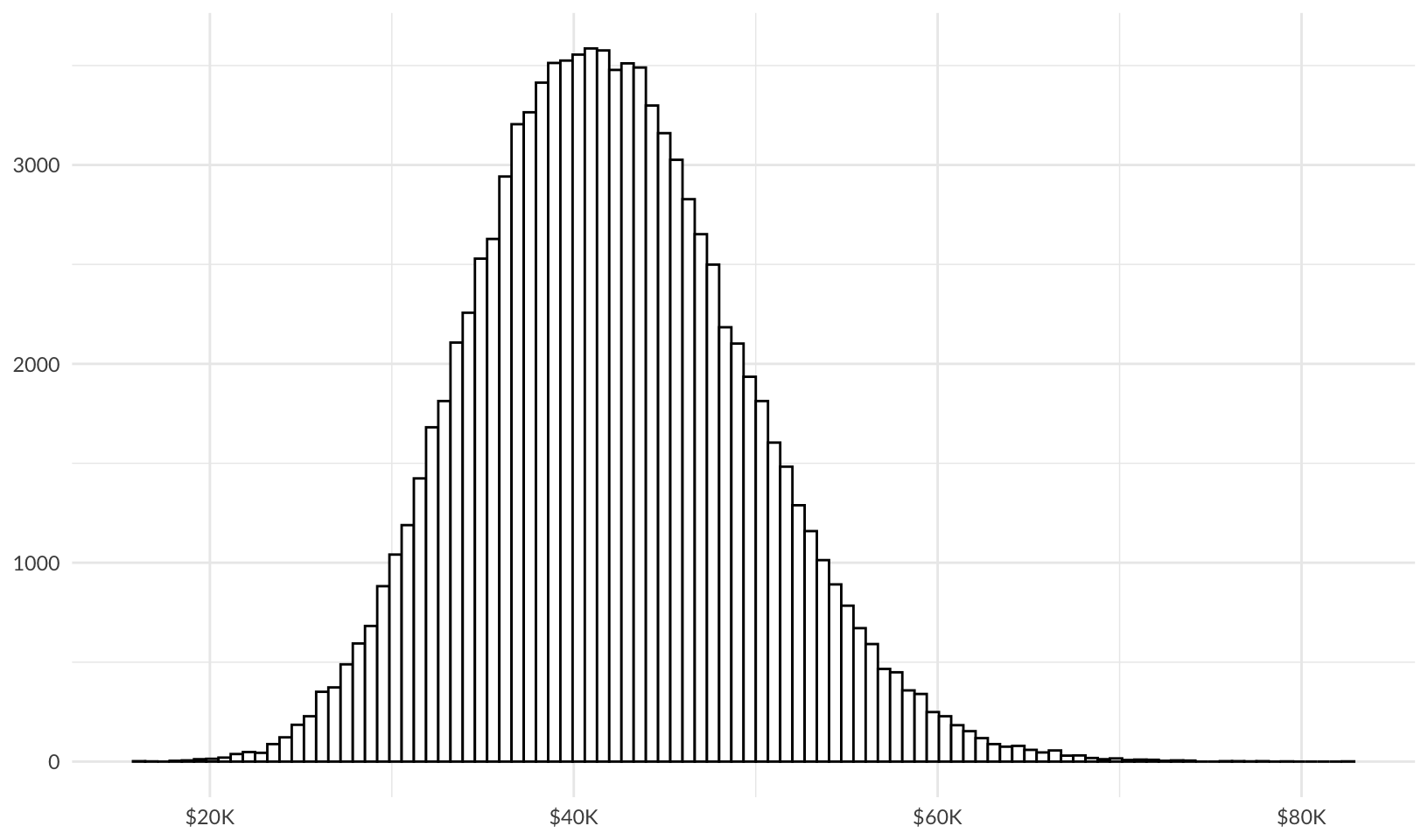
summary(baseline_malware) year risk treatment events
Min. : 1 Length:25000 Length:25000 Min. :26
1st Qu.: 6251 Class :character Class :character 1st Qu.:47
Median :12500 Mode :character Mode :character Median :52
Mean :12500 Mean :52
3rd Qu.:18750 3rd Qu.:57
Max. :25000 Max. :84
losses
Min. :13847
1st Qu.:36903
Median :41723
Mean :42056
3rd Qu.:46823
Max. :75203 In this case, the baseline risk is never 0, and falls within a range of about $15K to $80K, with a typical cost of $40K/year.
What is the value of reducing the likelihood of malware by 50%?
impact_malware <- calc_risk("impact malware", lambda = 26, meanlog = 6.44961, sdlog = 0.6999362)
impact_malware_return <-
full_join(baseline_malware, impact_malware, by = "year", suffix = c("_base", "_reduced")) |>
select(c("year", "losses_base", "losses_reduced")) |>
mutate(return = losses_base - losses_reduced)
summary(impact_malware_return) year losses_base losses_reduced return
Min. : 1 Min. :13847 Min. : 5297 Min. :-18724
1st Qu.: 6251 1st Qu.:36903 1st Qu.:17308 1st Qu.: 14890
Median :12500 Median :41723 Median :20657 Median : 20864
Mean :12500 Mean :42056 Mean :21019 Mean : 21037
3rd Qu.:18750 3rd Qu.:46823 3rd Qu.:24324 3rd Qu.: 27051
Max. :25000 Max. :75203 Max. :46374 Max. : 65892 impact_malware_return |>
pull(return) |>
quantile(0.01) 1%
-100.9249 While there are still cases where investing in security generates a negative return, over 99% of the time, the return is positive, with an average return of just over $20,000. In this hypothetical example, $20K/year isn’t a big deal, which leads me to conclude that the entertainment company Marcus was working with had a much higher baseline rate of malware incidents, saw a much larger reduction, and probably spent more on typical response.
So, security can be a good investment, if it reduces the likelihood and/or impact of frequent events, like malware response.
Appendix
Work out how to reduce impact by 50% through trial and error, with hints from Google AI:
base <- rlnorm(1e7, meanlog, sdlog)
reduced <- rlnorm(1e7, meanlog - log(2), sdlog)
base_sum <- summary(base)
reduced_sum <- summary(reduced)
base_sum Min. 1st Qu. Median Mean 3rd Qu. Max.
0.000e+00 3.585e+04 2.842e+05 3.119e+07 2.257e+06 2.536e+12 reduced_sum Min. 1st Qu. Median Mean 3rd Qu. Max.
0.000e+00 1.797e+04 1.426e+05 1.542e+07 1.131e+06 1.031e+12 base_sum / reduced_sum Min. 1st Qu. Median Mean 3rd Qu. Max.
2.044 1.995 1.992 2.023 1.996 2.459 meanlog - log(2) does appear to be the best way of cutting impact in “half”; the first quartile, median, mean, and 3rd quartile are all reduced by approximately half. This is identical to the original approach since -log(2) == log(0.5), but is a bit clearer (divide by 2 vs multiply by 0.5).