SRA Workshop 7

Working notebook for SRA 2021 Workshop 7, “Monte Carlo simulation and probability bounds analysis in R with hardly any data (Instructors: Ferson & Grey)”

library(MASS)
library(sn)

Instructions

Download sra.r and pba.r from https://sites.google.com/site/hardlyanydata and source it into R. Set RStudio = TRUE for use within RStudio and save the file. The library also requires the package sn. Use rm(list = ls()) to clear R environment.

There is another version of pba.r on GitHub

Monte Carlo

Monte Carlo example from class using sra.R; contaminant plume (from Lobascio), slide 37-39 in the workshop PowerPoint:

View the cumulative probability plot by entering the letter in the console.

source("assets/sra.R")

## :sra> library loaded

# nolint start
L <- uniform(80, 120) # [m], source-receptor distance
i <- uniform(0.0003, 0.0008) # [], hydraulic gradient
K <- lognormal(1000, 750) # [m yr1], hydraulic conductivity
n <- lognormal(0.25, 0.05) # [], effective soil porosity
BD <- lognormal(1650, 100) # [kg per m3], soil bulk density
foc <- uniform(0.0001, 0.005) # fraction organic carbon
Koc <- normal(10, 3) # [m3 per kg], partition coefficient

T <- (n + BD * foc * Koc) * L / (K * i) # all variables assumed independent
summary(T)

## 
## Monte Carlo distribution summary
##   Mean: 13036.42
##   Variance: 244795478
##   Std Deviation: 15645.94
##   Width of interquartile range: 12919.15
##   Width of overall range: 382290.3
##   Order statistics
##      Left (min) value: -1430.177
##      1st percentile: 337.4495
##      5th percentile: 943.1102
##      25th percentile: 3689.254
##      Median (50th%ile): 8200.185
##      75th percentile: 16608.4
##      95th percentile: 41416.06
##      99th percentile: 72003.67
##      Right (max) value: 380860.1
##   Replications: 20000

T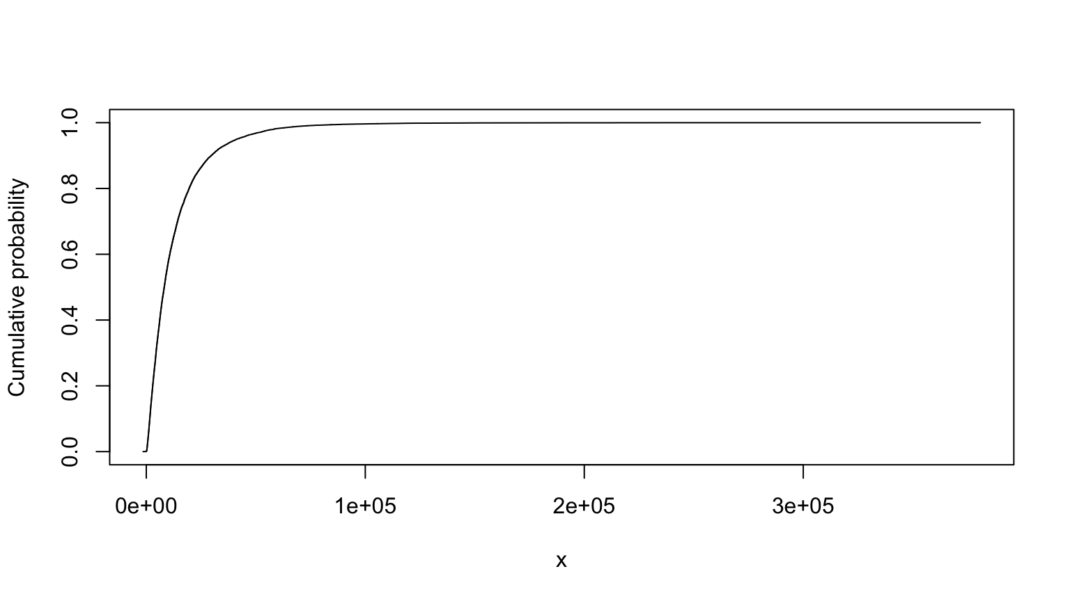

## MC (min=-1430.1767825287, median=8200.18534813244, mean=13036.4229606936, max=380860.074154619)

# nolint end

Truncated version, from slide 40:

# nolint start
L <- uniform(80, 120) # [m], source-receptor distance
i <- uniform(0.0003, 0.0008) # [], hydraulic gradient
K <- lognormal(1000, 750) # [m yr1], hydraulic conductivity
K <- truncate(K, 300, 3000)
n <- lognormal(0.25, 0.05) # [], effective soil porosity
n <- truncate(n, 0.2, 0.35)
BD <- lognormal(1650, 100) # [kg per m3], soil bulk density
BD <- truncate(BD, 1500, 1750)
foc <- uniform(0.0001, 0.005) # fraction organic carbon
Koc <- normal(10, 3) # [m3 per kg], partition coefficient
Koc <- truncate(Koc, 5, 20)

T <- (n + BD * foc * Koc) * L / (K * i)
summary(T)

## 
## Monte Carlo distribution summary
##   Mean: 12243.63
##   Variance: 158328719
##   Std Deviation: 12582.87
##   Width of interquartile range: 12515.5
##   Width of overall range: 128412.6
##   Order statistics
##      Left (min) value: 89.03806
##      1st percentile: 387.9319
##      5th percentile: 1021.713
##      25th percentile: 3795.62
##      Median (50th%ile): 8151.298
##      75th percentile: 16311.12
##      95th percentile: 37662.01
##      99th percentile: 59407.54
##      Right (max) value: 128501.7
##   Replications: 20000

T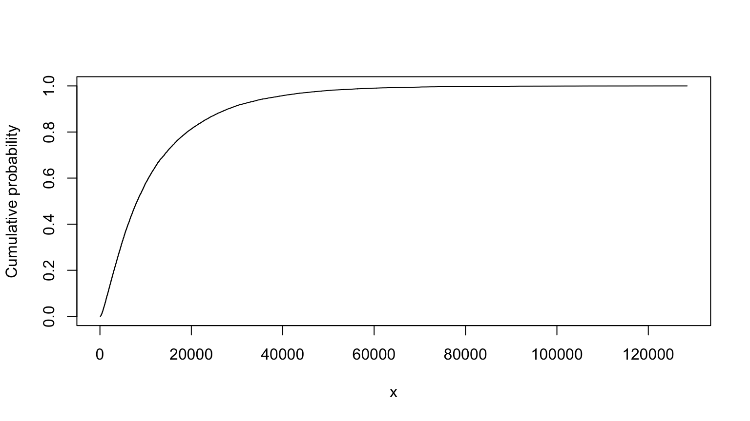

## MC (min=89.0380601528359, median=8151.29820845253, mean=12243.6319738417, max=128501.666854059)

# nolint end

Maximum entropy version, from slide 70:

T and Tind are pretty similar. In this case, the maximum entropy approach comes up with a similar distribution as the truncated approach.

# nolint start
L <- MEmmms(80, 120, 100, 11.55) # source-receptor distance
i <- MEmmms(0.0003, 0.0008, 0.00055, 0.0001443) # hydraulic gradient
K <- MEmmms(300, 3000, 1000, 750) # hydraulic conductivity
n <- MEmmms(0.2, 0.35, 0.25, 0.05) # effective soil porosity
BD <- MEmmms(1500, 1750, 1650, 100) # soil bulk density
foc <- MEmmms(0.0001, 0.005, 0.00255, 0.001415) # fraction organic carbon
Koc <- MEmmms(5, 20, 10, 3) # organic partition coefficient

Tind <- (n + BD * foc * Koc) * L / (K * i)
summary(Tind)

## 
## Monte Carlo distribution summary
##   Mean: 14008.97
##   Variance: 228701339
##   Std Deviation: 15122.87
##   Width of interquartile range: 15340.24
##   Width of overall range: 134412.2
##   Order statistics
##      Left (min) value: 93.35144
##      1st percentile: 348.8692
##      5th percentile: 992.8687
##      25th percentile: 3711.77
##      Median (50th%ile): 8642.153
##      75th percentile: 19052.01
##      95th percentile: 45542.41
##      99th percentile: 69871.42
##      Right (max) value: 134505.6
##   Replications: 20000

Tind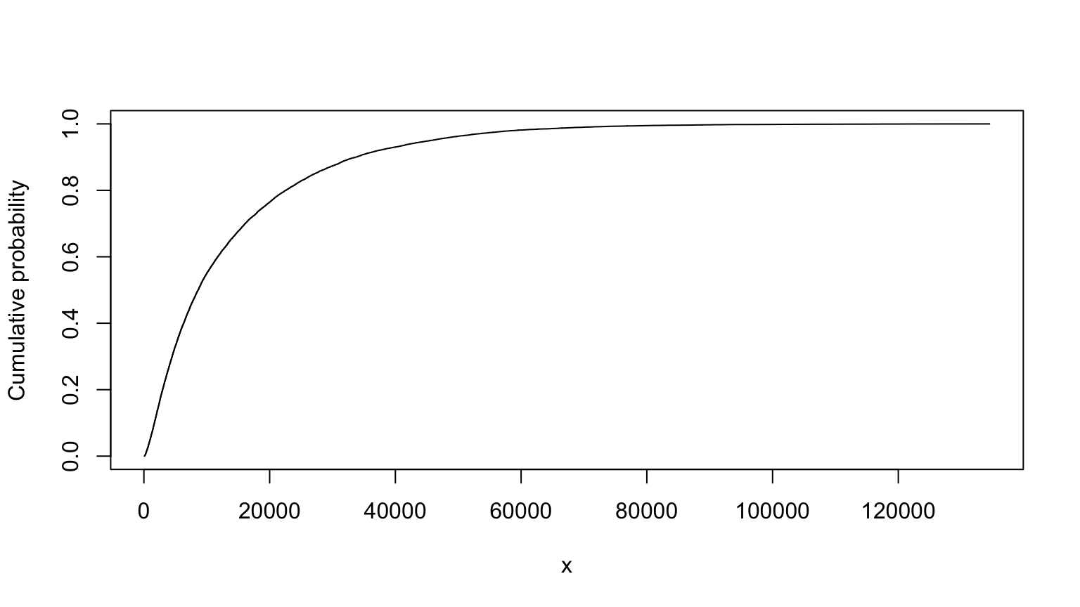

## MC (min=93.3514369431351, median=8642.15281492068, mean=14008.9725287954, max=134505.588523945)

# nolint end

Probability Bounds Analysis

Conduct the same analysis using PBA, from slide 162. See the important note from slide 162 below.

Note: N.B. The implementation of mmms in pba.r is incomplete so, while its results are bounds, they are not best possible bounds

# ideally we'd clear the environment with `rm(list = ls())`, but that doesn't work here;
# an alternative would be to move this to a separate notebook. This approach appears to be OK,
# outputs from running just the setup and the entire notebook are the same.

# this code breaks build_analysis_site() - commented out because of that.
# uncomment this code and it should work within the notebook in RStudio.
# nolint start
# source("assets/pba.R")
#
# L <- mmms(80, 120, 100, 11.55) # source-receptor distance
# i <- mmms(0.0003, 0.0008, 0.00055, 0.0001443) # hydraulic gradient
# K <- mmms(300, 3000, 1000, 750) # hydraulic conductivity
# n <- mmms(0.2, 0.35, 0.25, 0.05) # effective soil porosity
# BD <- mmms(1500, 1750, 1650, 100) # soil bulk density
# foc <- mmms(0.0001, 0.005, 0.00255, 0.001415) # fraction organic carbon
# Koc <- mmms(5, 20, 10, 3) # organic partition coefficient
#
# up <- 100000 # detail
# Tind <- (n + BD * foc * Koc) * L / (K * i)
# Tind <- pmin(Tind, up)
#
# summary(Tind)
# Tind
# nolint end