library(palmerpenguins)
library(ggplot2)
library(ggthemes)
library(showtext)
library(cranlogs)
library(dplyr)R Books
reading
An actively maintained and curated list of R Books and other recommended resources from my reading list.
Libraries
Libraries used in this notebook.
Getting Started
Books and resources I recommend for learning R.
R for Data Science
R for Data Science (2e) - Second Edition of Hadley Wickham’s introductory book on R and exploratory data analysis. The book contains example code and exercises in most chapters. I used the first edition as my primary source when I was first learning R, and still recommend the book for beginners who want to learn R. The book teaches the basics of using tidyverse R1 for exploratory data analysis and visualization. A companion book provides suggested solutions to the exercises.
Sample visualization from the first chapter:
# visualization from https://r4ds.hadley.nz/data-visualize#first-steps
ggplot(
  data = penguins,
  mapping = aes(x = flipper_length_mm, y = body_mass_g)
) +
  geom_point(aes(color = species, shape = species)) +
  geom_smooth(method = "lm") +
  labs(
    title = "Body mass and flipper length",
    subtitle = "Dimensions for Adelie, Chinstrap, and Gentoo Penguins",
    x = "Flipper length (mm)", y = "Body mass (g)",
    color = "Species", shape = "Species"
  ) +
  scale_color_colorblind()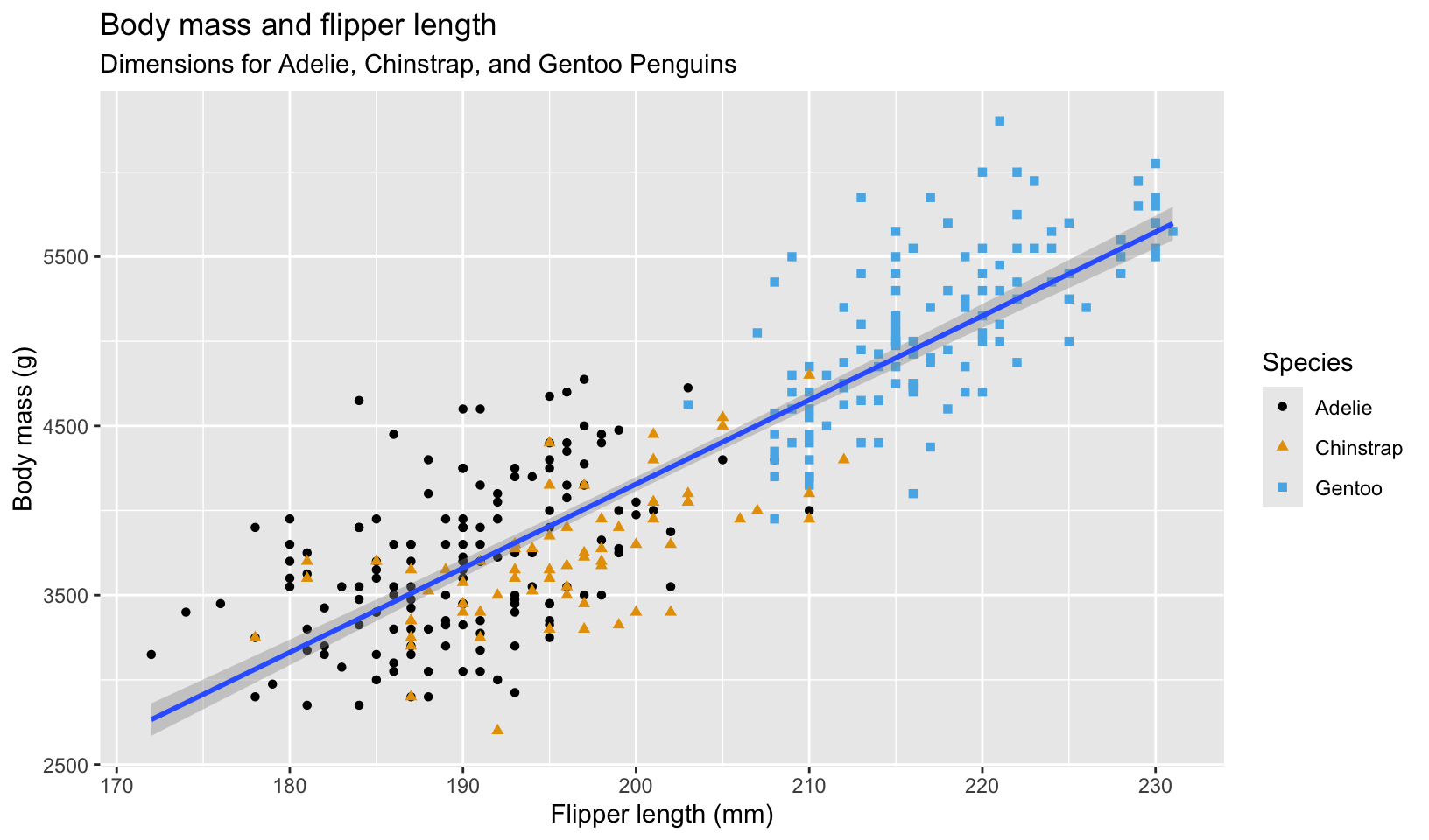
Resources
In addition to R for Data Science, I recommend the following resources for new R users:
- The R Graph Gallery - library of charts made with R and ggplot2
- Packages for writing better code:
- Style guides for writing better code:
- tidyverse style guide - implemented by styler
- Google’s R Style Guide - a fork of the tidyverse guide
rdev, my personalized collection of R development tools, includes all three of these packages and more, along with my own style guide and R environment setup instructions.
Custom Fonts
Working with custom fonts in R can be problematic, and font support is platform-dependent. By default, R provides default mappings for three device-independent font families: sans (Helvetica or Arial), serif (Times New Roman), and mono (Courier New). On macOS, quartz is the default graphics device, and uses the following fonts:
quartzFonts()$serif
[1] "Times-Roman" "Times-Bold" "Times-Italic" "Times-BoldItalic"
$sans
[1] "Helvetica" "Helvetica-Bold" "Helvetica-Oblique"
[4] "Helvetica-BoldOblique"
$mono
[1] "Courier" "Courier-Bold" "Courier-Oblique"
[4] "Courier-BoldOblique"Custom fonts installed on the local system should work without installing any additional packages:
size <- 28

ggplot() +
  annotate("text", x = 0, y = 0, label = "Default", size = size) +
  annotate("text", x = 0, y = -1, label = "Lato", family = "Lato", size = size) +
  annotate("text", x = 0, y = -2, label = "Metropolis", family = "Metropolis", size = size) +
  scale_y_continuous(limits = c(-2.5, 0.5)) +
  theme_void()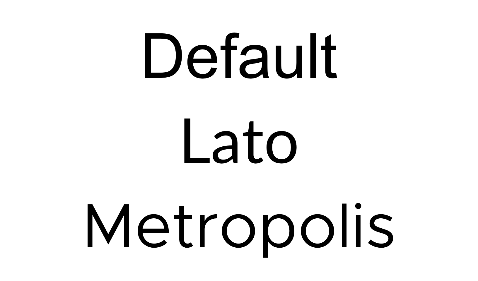
This approach works, but isn’t portable as it introduces hidden dependencies on the custom fonts. The plot above works because I have the Lato and Metropolis fonts installed on the macOS system I use to build this page; on systems without these fonts installed this plot would generate warnings and fallback to the default font:
ggplot() +
  annotate("text", x = 0, y = 0, label = "Not Missing", size = size) +
  annotate("text", x = 0, y = -1, label = "Missing", family = "missing", size = size) +
  scale_y_continuous(limits = c(-1.5, 0.5)) +
  theme_void()
Warning in grid.Call.graphics(C_text, as.graphicsAnnot(x$label), x$x, x$y, : no
font could be found for family "missing"
Warning in grid.Call.graphics(C_text, as.graphicsAnnot(x$label), x$x, x$y, : no
font could be found for family "missing"
Warning in grid.Call.graphics(C_text, as.graphicsAnnot(x$label), x$x, x$y, : no
font could be found for family "missing"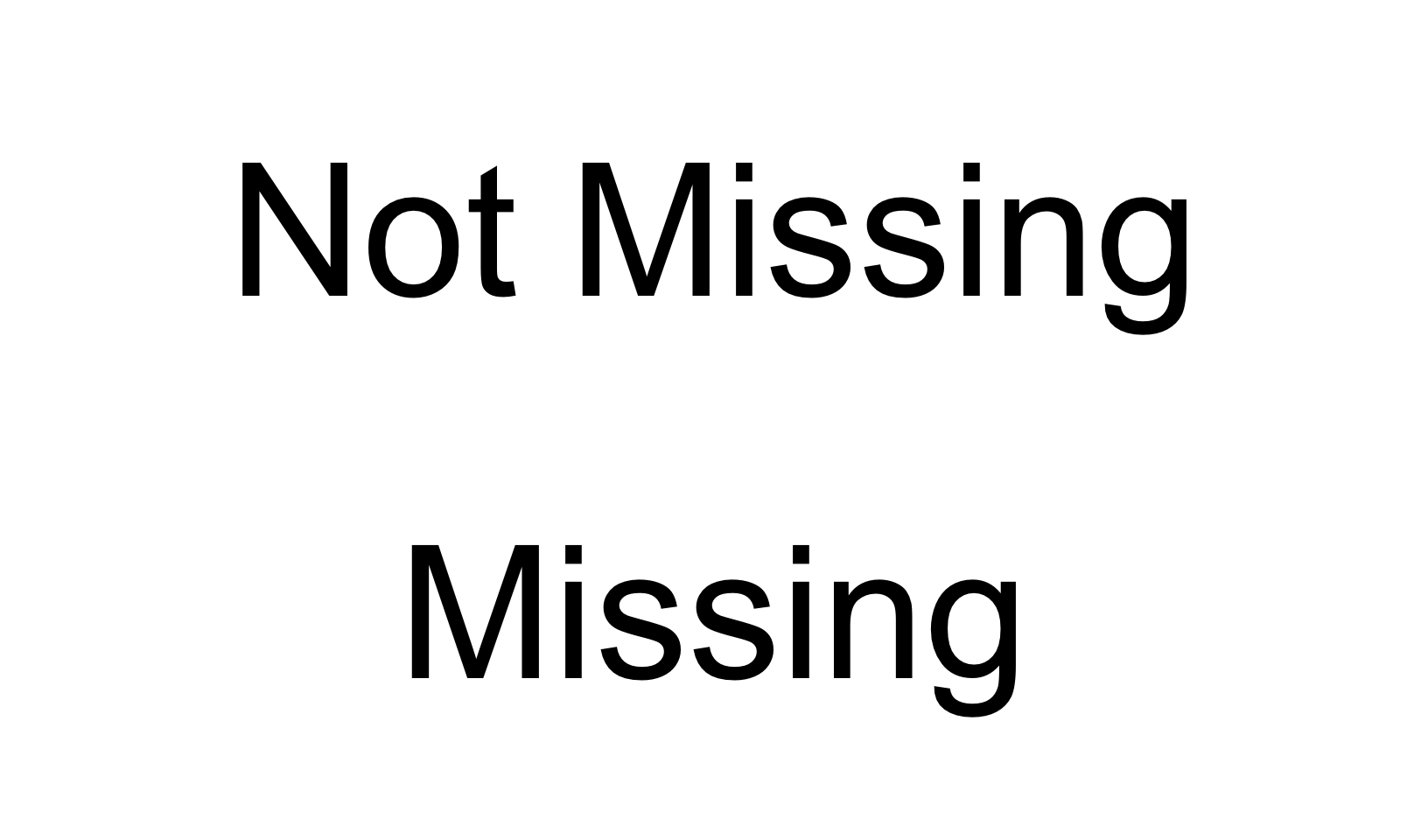
There are a few packages that facilitate use of custom fonts in R:
- extrafont is an older package that can import fonts for use in PDF, PostScript, and Windows
- showtext is a newer package that is most often recommended for custom fonts, and can import fonts directly from Google Fonts with
font_add_google() - ragg is a graphics back-end that gives access to all installed system fonts, and is recommended as an alternative to showtext
- systemfonts locates installed fonts using system libraries on macOS and Linux, and Freetype on Windows
On macOS, no additional packages are needed to access all system fonts, although this may not be the case on other platforms (I haven’t tested). I currently use a combination of base R and showtext. systemfonts can help troubleshoot issues by showing what system fonts R recognizes.
showtext will work even with fonts not present on the local system:
font_add_google("Open Sans")
showtext_auto()

ggplot() +
  annotate("text", x = 0, y = 0, label = "Default", size = size) +
  annotate("text", x = 0, y = -1, label = "Open Sans", family = "Open Sans", size = size) +
  scale_y_continuous(limits = c(-1.5, 0.5)) +
  theme_void()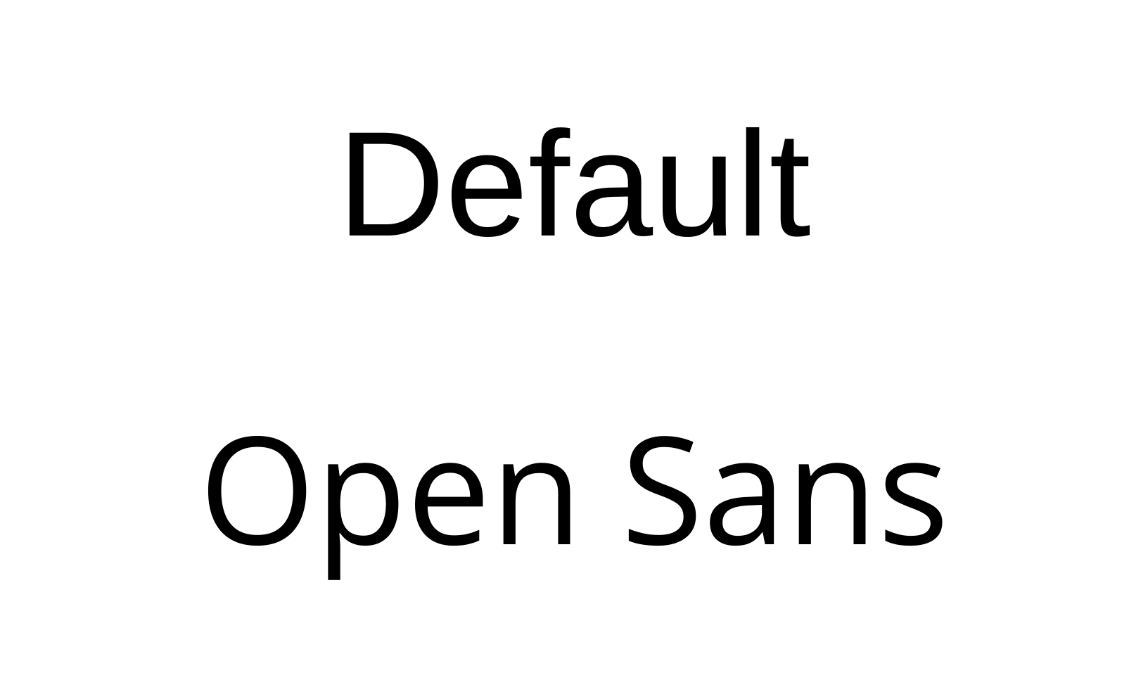
An important caveat: showtext replaces all system fonts when enabled. To disable it and use the standard font system, run:
showtext_auto(FALSE)Additional articles on using custom fonts in R:
Additional Reading
Books I read to improve my knowledge of R.
- R Packages (2e) - the second edition of Hadley Wickham’s book on writing R packages, which I used to build rdev
- Advanced R - the second edition of Hadley’s book on R programming, which explains the R language (the first edition uses more base R than the second edition)
- Advanced R Solutions - solutions to exercises from Advanced R
- ggplot2: Elegant Graphics for Data Analysis (3e) - the third edition of Hadley’s book on his implementation of Leland Wilkinson’s Grammar of Graphics
- Solutions to ggplot2: Elegant Graphics for Data Analysis - solutions to exercises from ggplot2
My own notes and solutions to the Advanced R and ggplot2 exercises are available on this site.
raps-with-r
Building reproducible analytical pipelines with R - the stated goal of the book is to improve the reproducibility of data analysis. I don’t recommend this book. Section 1 is a reasonably good introduction to git and GitHub, but introduces trunk-based development without covering linear commit history. Section 2 provides some good advice, but much that I disagree with, including inline use of knitr::knit_child to automate creation of sections (which break the notebook workflow) and fusen to create packages from .Rmd files, which I found to create extra work with no clear benefits over using and/or extending the standard package layout like vertical or my own layout from rdev. (Interestingly, the author of vertical is also switching to Quarto for reproducible research and analysis) I also found the code examples to be inconsistent and a bit clunky.
Chapter 12 gives recommendations on testing: unit testing with some basic examples, assertive programming, Test-Driven Development (TDD), and test coverage. It suggests three packages for R assertions: assertthat, chk, and checkmate. Both chk and checkmate are designed to check function arguments; of the two, checkmate appears to be more robust and built to address the downside of R being a dynamically typed language.
For data validation, I currently use stopifnot(), although I may switch to either assertr or validate, which are both popular packages. I validate function arguments using manual checks, but checkmate looks appealing as a way to write more succinct code. Total downloads for the assertr, validate, chk, and checkmate packages for the last month are listed below:
cran_downloads(
  packages = c("assertr", "validate", "chk", "checkmate"),
  when = "last-month"
) |>
  group_by(package) |>
  summarize(downloads = sum(count), as_of = max(date))
# A tibble: 4 × 3
package downloads as_of
<chr> <dbl> <date>
1 assertr 2801 2026-03-30
2 checkmate 495751 2026-03-30
3 chk 21189 2026-03-30
4 validate 2103 2026-03-302023-12-29 Update: I’ve started using checkmate to check function arguments and have found that validate is better overall at data validation.
Chapter 13 introduces targets, “a Make-like pipeline tool for statistics and data science in R.” Conceptually, targets is very similar to an R Notebook, but like Make, will skip components that are up to date, and can run targets in parallel to speed up builds. targets can also render R Markdown documents using the tarchetypes package. I found the example target pipeline in the book convoluted and didn’t attempt to follow it. The targets manual explains that it implements two kinds of literate programming:
- A literate programming source document (or Quarto project) that renders inside an individual target. Here, you define a special kind of target that runs a lightweight R Markdown report which depends on upstream targets.
- Target Markdown, an overarching system in which one or more Quarto or R Markdown files write the _targets.R file and encapsulate the pipeline.
Of these two types, the second is a better fit with my preferred workflow: including multiple self-contained notebooks in a single repository. From the appendix, the design of Target Markdown supports both interactive development using notebooks and running a pipeline non-interactively when rendering the final document. For my work, targets doesn’t offer significant advantages over using R Markdown and Quarto - the only slowdown I typically encounter is when building a site with many notebooks, which the Quarto freeze option handles by only re-rendering documents when the source file changes. (I’m not performing the large, complex computations that targets is designed for)
Chapter 14 covers Docker, and asserts that it is necessary for reproducibility. While using Docker ensures a stable operating system environment, I think the book overstates the case for reproducibility, citing a single example where the operating system changed the results of an analysis because the scripts relied on OS file ordering. Much like use of targets, Docker would be most useful for projects with complex development environments shared across teams, but much of the benefits can be achieved using other approaches, like using OS-independent code. The chapter also encourages using a “frozen” development environment that is updated on a fixed schedule to minimize the impact of frequent updates. This is exactly the opposite of the modern DevOps approach - the issues created by small, frequent updates are smaller and easier to address than the more complex problems created by large upgrades. I always start development by updating packages to the latest production release - while this sometimes introduces issues, they are typically easy to fix, and prioritizing maintenance first improves quality and security.
An alternate approach to using Docker is to leverage GitHub Actions, which provides on-demand virtual machines that can be used to consistently test, build, and deploy code. The Tidyverse community provides a library of GitHub Actions for R, which I’ve customized for rdev. In fact, chapter 15 covers use of GitHub Actions using r-lib and presents them as a potential alternative for Docker.
Overall, I do follow the book’s core recommendations for reproducibility:
- Use version control extensively
- Use trunk-based development
- Adopt functional programming and DRY
- Use R Markdown which embeds analysis code and code output directly into the written report
- Use renv to manage dependencies
- Package all R code and publish using GitHub Pages
- Write unit tests using testthat
- Use assertions to validate function arguments and imported data
- Check test coverage using
covr - Use automated builds (but using Quarto instead of targets)
I would consider use of targets and Docker for larger, more complex, or long-lived projects, but I found that fusen offered no clear benefits and wouldn’t recommend its use. I think the biggest lesson I took from the book was to follow DRY a bit more strictly than I currently do, and use more functions, tests, and assertions in my analysis code.
The book does reference some interesting reading I’ve added to my list:
- John M. Chambers. “Object-Oriented Programming, Functional Programming and R.” Statist. Sci. 29 (2) 167 - 180, May 2014. https://doi.org/10.1214/13-STS452
- Trunk-Based Development And Branch By Abstraction
While reading the book, I discovered some interesting additional resources:
- Vertical, a “an R-based structured workflow for creating and sharing research assets in the form of an extended R package”, which I plan to review and compare to rdev
- Four ways to write assertion checks in R - an article on four methods for writing assertions in R:
- Use
stopifnot()from base R - Use the
assertthatpackage (last updated March 2019) - Use the
assertivepackage (last updated July 2020) - Use the
assertrpackage for data assertions, which works especially well for assertion checks against data frames used in data analysis
- Use
- I also revisited the
validatepackage, a data validation rules engine, which includes the Data Validation Cookbook (in Future Reading)
rstats.wtf
What They Forgot to Teach You About R - a book based on a workshop taught by current and former posit employees intended for self-taught data analysts. It’s short, still in draft, and offers good advice on R development (I use almost all the suggestions):
- Use an IDE (RStudio)
- Don’t save
.RData - Restart R frequently
- Automate long workflows using targets
- Don’t use
setwd() - Use RStudio projects
- Use here and fs for paths
- Use “-” as space and “_” as a field delimiter in file names
- Use ISO standard dates (ISO 8601, YYYY-MM-DD)
- Use version control (git, GitHub)
- Use renv, rig, and homebrew
- Use
.Renvironand.Rprofile - Use CRAN R and CRAN binaries to speed up package installation
- Don’t use Conda (for Python)
- Update packages!
- Use debugging commands and RStudio for troubleshooting
- Search for error messages and read the source code to understand your problem
The book also suggests use of the Posit Public Package Manager (P3M). I’d like to agree with this advice, however, I’ve had problems with their binaries; this package (rtraining) doesn’t work when using P3M, and works fine with CRAN binary packages.
do4ds
DevOps for Data Science, another book written by a Posit employee was brought to my attention thanks to a LinkedIn Post by @Corey Neskey (It included a reference to rstats.wtf, which I read first). The book is split into 3 sections:
- DevOps Lessons for Data Science (Chapters 1-6)
- IT/Admin for Data Science (Chapters 7-14)
- Enterprise-Grade Data Science (Chapters 15-18)
I chose not to do the exercises in the book.
Chapters 1-6 cover basic software engineering concepts including library/package management, the three-tier application model, types of projects (jobs, apps, reports, and APIs), connecting to databases and APIs, logging and monitoring, deploying code with CI/CD in dev, test, and production (including branching strategy) and Docker.
Useful references from the first section include:
- pins, a package for publishing data, models, and other R objects to folders or cloud storage, including AWS, Azure, GCP, Google Drive, OneDrive, and Dropbox.
- vetiver, R and Python libraries designed to version, deploy, and monitor a trained ML model.
- Mastering Shiny, Hadley Wickham’s book on R Shiny, published in 2021.
Chapters 7-14 cover basic infrastructure engineering concepts, including cloud computing (IaaS, PaaS, and SaaS), the command line (terminals, shells, and SSH), Linux (Unix), scaling hardware, networking, DNS, and TLS (HTTPS).
I disagreed with the recommendations on macOS terminals and configuration management in chapter 8; I use macOS Terminal and .zprofile and .zshrc respectively. Given my background in infrastructure and systems engineering, most of the section was not new to me, except for AWS, which I haven’t worked with.
There was one useful reference from the second section:
- paws, an Amazon Web Services SDK for R.
Chapters 15-18 cover issues that come up in larger, “enterprise”, organizations. It includes discussion of networking and network security (including proxies), authentication and authorization (including identity and access management: LDAP, SSO, MFA, RBAC and ABAC), infrastructure as code, Docker and Kubernetes, and how enterprise policies affect use of R and Python packages.
The third section doesn’t contain labs, and has one useful reference:
- httr2, tools for creating and modifying HTTP requests, then performing them and processing the results.
Future Reading
R books on my reading list.
- The R Manuals - a re-styled version of the original R manuals, published using Quarto (starting with Writing R Extensions)
- R Markdown: The Definitive Guide - written by the author of knitr
- R Markdown Cookbook - the follow-up to The Definitive Guide
- The Data Validation Cookbook - a book on the R validate package
- Discovering Statistics Using R - recommended to me as an introduction to statistics using R
- While it’s not an R book, I am interested in using DiagrammeR for graph visualizations (it also supports Graphviz and Mermaid)
R Dialects
An explanatory note on the R dialects of base R and tidyverse R.
The R programming language is over 30 years old and has a large number of packages (R libraries) that extend R. Unlike python (a general purpose language), R was designed specifically for analysis, visualization, and statistical modeling, which is why I chose R for data analysis: it has built-in support for data structures like data frames (implemented in python using pandas), vectors, packages for just about any statistical tool you’d need, and of course, ggplot2. In fairness, python is more popular, more robust, and a better tool for some tasks, like data acquisition and machine learning (which were not priorities for my use).
Like many human languages, R has developed two distinct dialects: base R and tidyverse R. Base R consists of the packages included in the R distribution (base, compiler, datasets, graphics, grDevices, grid, methods, parallel, splines, stats, stats4, tcltk, tools, utils), and the Tidyverse is a collection of packages that implement a domain-specific language for data analysis, originally created by Hadley Wickham.
In my experience, tidyverse R is better for data analysis, where base R is better for writing packages - tidyverse functions are closer to natural language, but have many more dependencies. Comparing two popular tools for data manipulation, dplyr (tidyverse R) and data.table (base R) shows these differences.
This code snippet is from a short analysis of survey responses using dplyr:
survey_results <- survey_import |>
  mutate(across(Q1:Q7, ~ case_when(
    .x == "strongly disagree" ~ 1,
    .x == "disagree" ~ 2,
    .x == "neither agree nor disagree" ~ 3,
    .x == "agree" ~ 4,
    .x == "strongly agree" ~ 5
  ))) |>
  mutate(Q8 = as.numeric(Q8 == "Yes")) |>
  arrange(end_date)
The code is reasonably easy to understand, even if you’re not familiar with R.
The same code written in data.table isn’t as clear:
likert_5 <- c(
  "strongly disagree", "disagree", "neither agree nor disagree",
  "agree", "strongly agree"
)
q_likert <- paste0("Q", 1:7)
q_yesno <- "Q8"

survey_results <- copy(survey_import)
survey_results <- survey_results[
  , (q_likert) := lapply(.SD, \(x) as.numeric(factor(x, levels = likert_5))),
  .SDcols = q_likert
][
  , (q_yesno) := lapply(.SD, \(x) as.numeric(x == "Yes")),
  .SDcols = q_yesno
][
  order(end_date)
]
While it may be harder to read, data.table has some clear advantages: it is quite fast, especially with very large datasets, and has no dependencies other than base R, where dplyr has many.
These tradeoffs are why I tend to use tidyverse R for analysis and base R for functions (most tidyverse expressions have functional equivalents in base R). Code used in data analysis should be clear and easy to read, which tidyverse R excels at. Packaged functions provide documentation and the source code isn’t typically read, but many dependencies can be problematic; R CMD check will raise a NOTE if there are too many imports.
Footnotes
For a detailed explanation of “tidyverse R”, see R Dialects↩︎