Hockey Cards Analysis

A simple Monte Carlo simulation in R, replicating Julia code from a LinkedIn post.

library(ggplot2)
library(jbplot)

Background

I came across an interesting post on LinkedIn that used Monte Carlo simulation to help answer the question “How much is a box of unopened Canadian hockey cards worth?” The example code was in Julia, and I wanted to recreate it in R for comparison.

Code

The base R code below is functionally equivalent to the Julia code, except it omits the trial ID in the result:

gretsky_cards <- function(trials) {
  set_cards <- 396
  carton_cards <- 672
  cartons <- 16
  box_cards <- carton_cards * cartons

  replicate(trials, {
    carton <- sample(1:set_cards, box_cards, replace = TRUE)
    sum(carton == 99)
  })
}

gretskys <- gretsky_cards(10000)

Also, instead of using a loop, I used replicate(), which I think is easier to use and understand.

Answer - Base R

Replicating the answer in base R:

summary(gretskys)

   Min. 1st Qu.  Median    Mean 3rd Qu.    Max. 
  10.00   23.00   27.00   27.17   31.00   51.00 

hist(gretskys)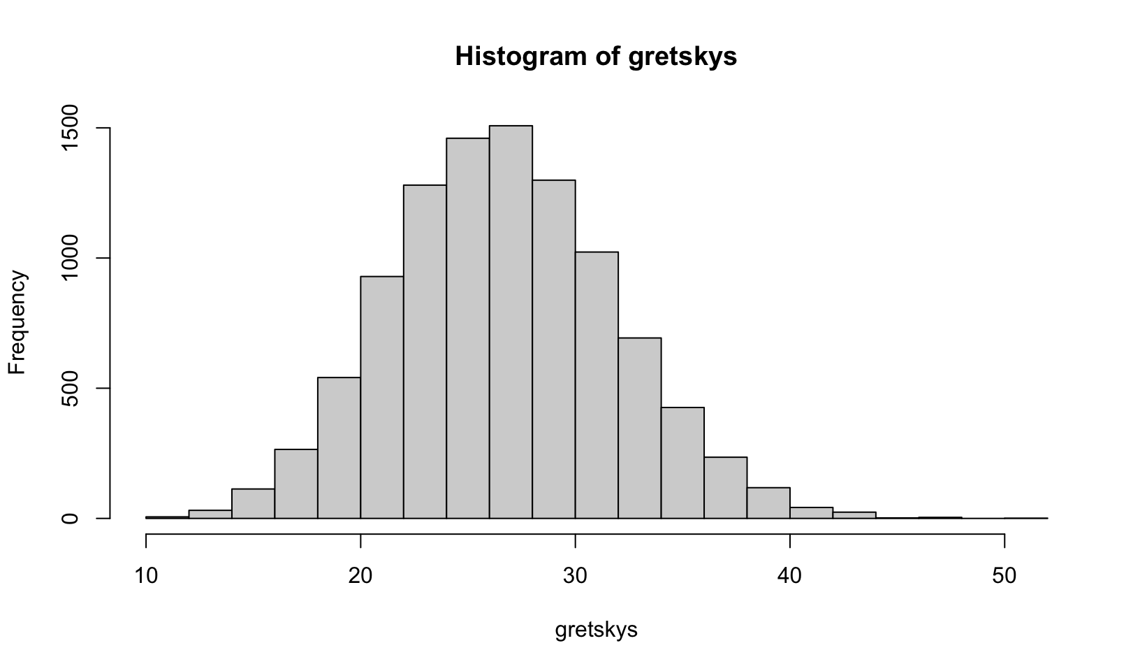

Answer - ggplot2

Use ggplot2 to create a prettier histogram:

ggplot(as.data.frame(gretskys), aes(gretskys)) +
  geom_hist_bw(binwidth = 1) +
  labs(title = "Gretsky cards per case", x = NULL, y = NULL) +
  labs(caption = "Number of occurrences over 10,000 simulations") +
  theme_quo()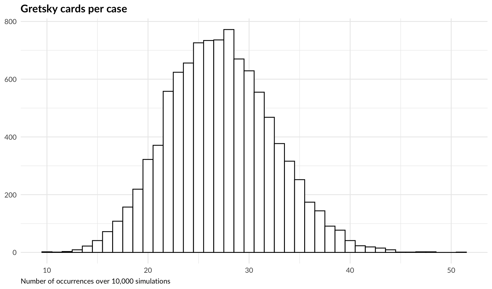

Performance

How does the performance compare to Julia?

bench::mark(gretsky_cards(10000))

Warning: Some expressions had a GC in every iteration; so filtering is
disabled.

# A tibble: 1 × 6
  expression                min   median `itr/sec` mem_alloc `gc/sec`
  <bch:expr>           <bch:tm> <bch:tm>     <dbl> <bch:byt>    <dbl>
1 gretsky_cards(10000)    2.44s    2.44s     0.410     1.2GB     13.9

In this case, it certainly appears to be slower than the Julia test result which was 1.63 seconds.