Professional services firm with $5M in annual revenue. A loss of 1% ($50K) is considered material.
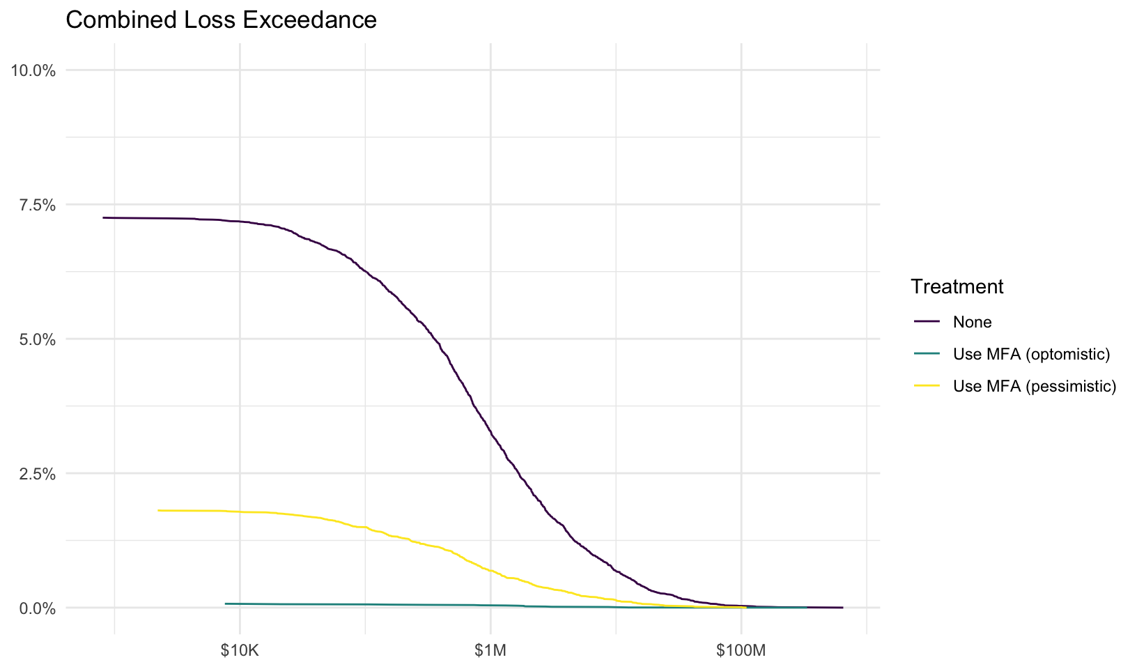
Supplementary Material from the Cyentia IRIS 2025 Report found that the likelihood of at least 1 incident in the next year is 7.48% for firms with less than $10M in revenue.
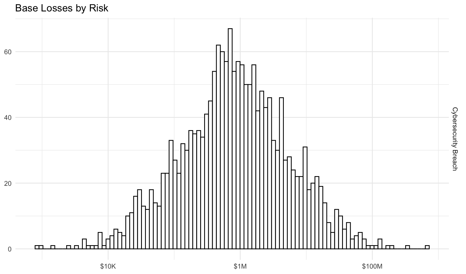
Figure A3 from the main IRIS 2025 Report shows that the median loss for the Professional sector is $736K and the 95th percentile is $17M. From this we use trial and error to calculate the 50% (median) loss at $31,900.
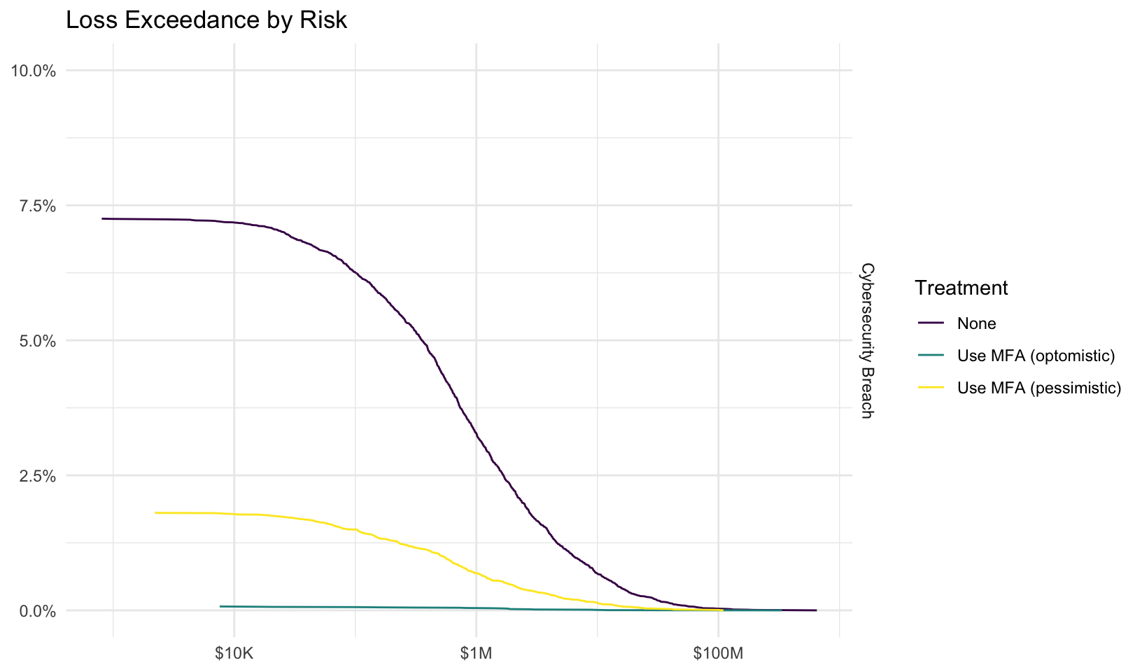
According to a preprint study, implementing MFA reduces the likelihood of compromise by 99%. An older study found that MFA reduced the likelihood of targeted attacks by 76%.
Note: the research on MFA looked at individuals, and other research on organizations found a lower reduction. For this analysis, we assume the individual risk reduction is achievable with a thorough and complete MFA implementation (fully implemented everywhere).
Import
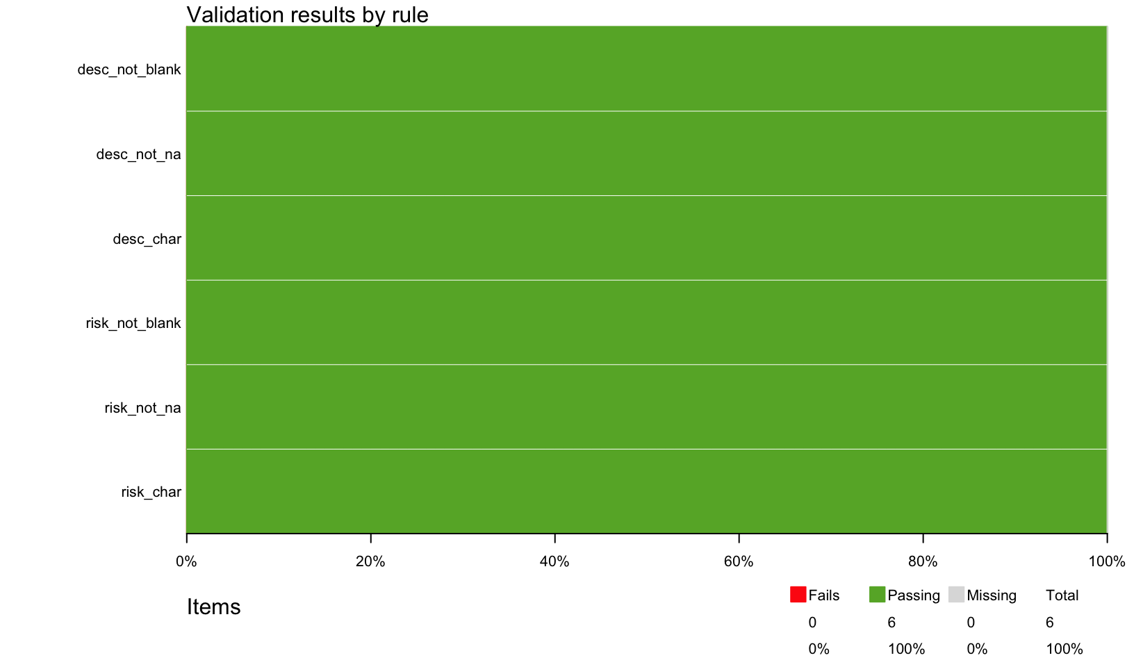
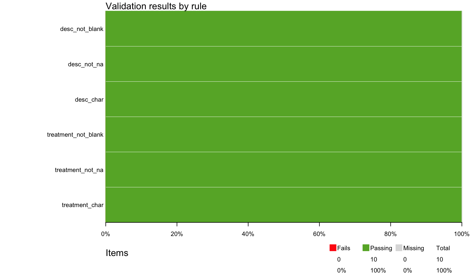
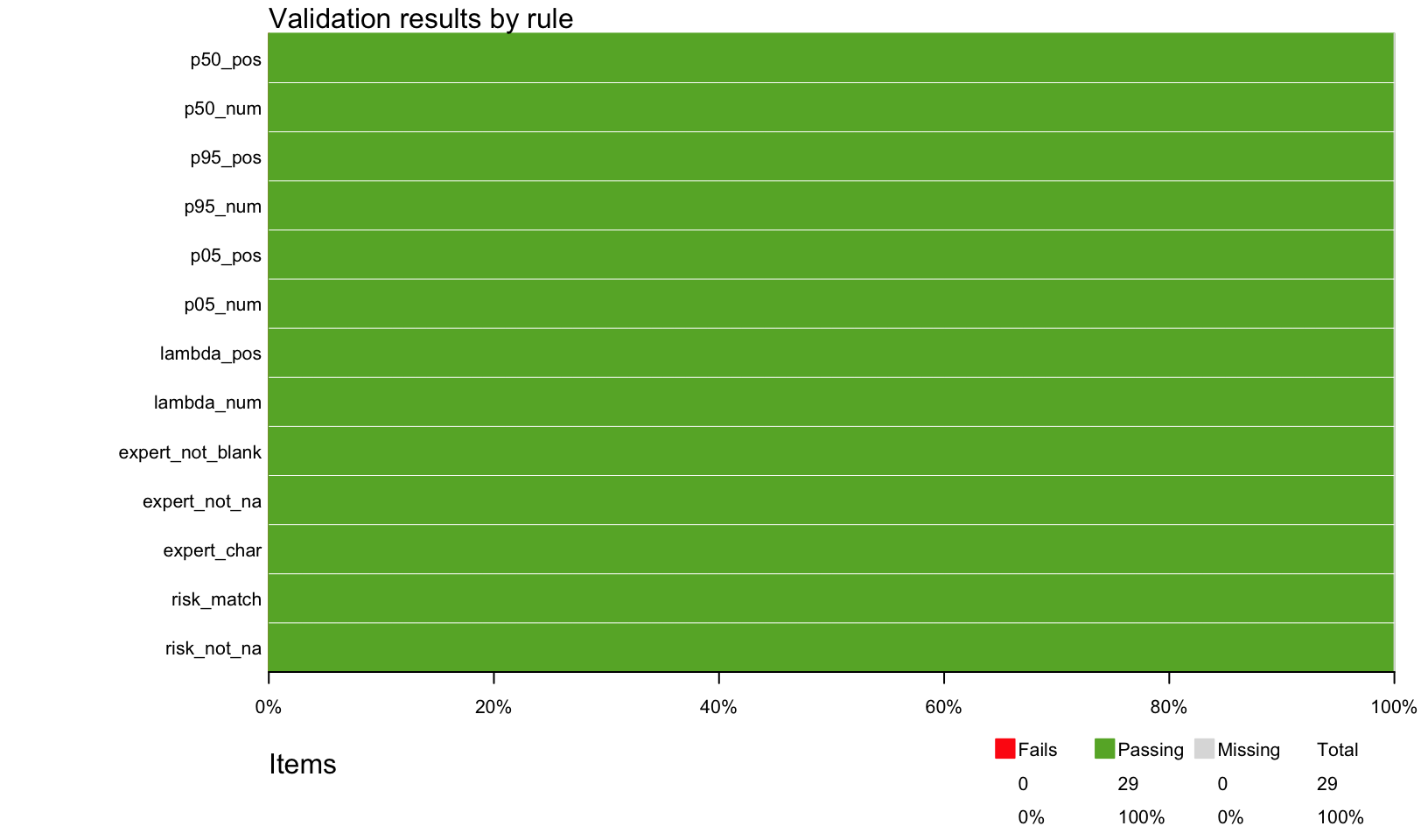
Import and validate data from Excel.
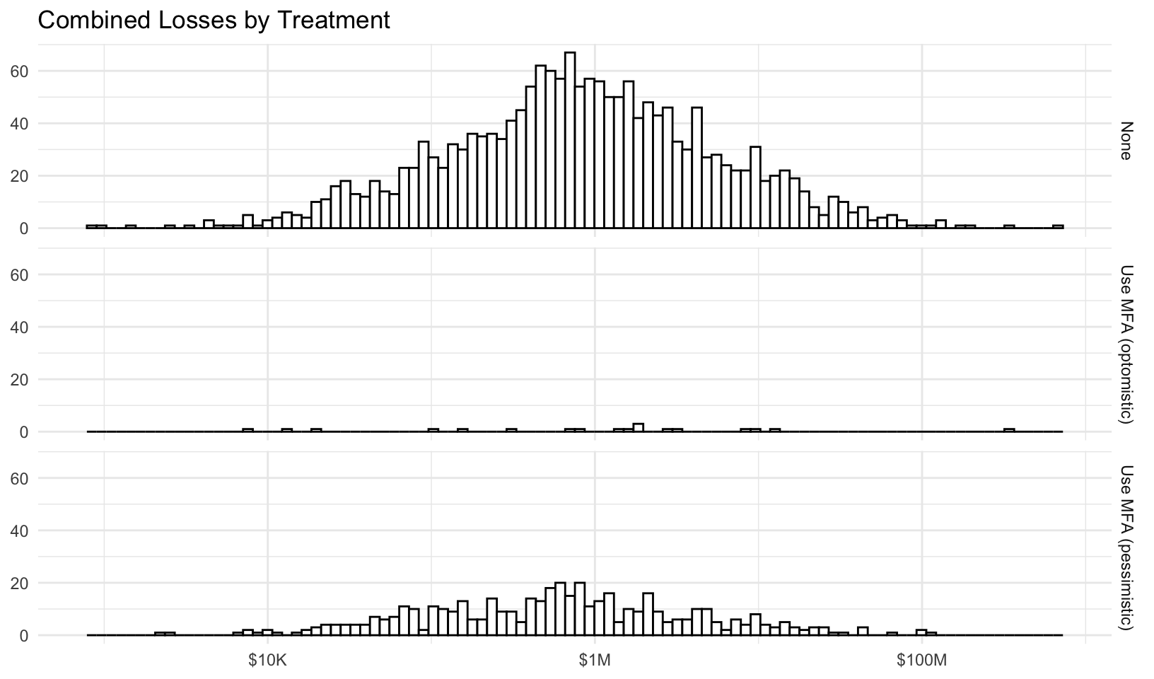
We use the IRIA 2025 data for the 5th, median, and 95th percentile of impact in all treatments, and adjust the frequency by 99% in the optimistic case and 76% in the pessimistic case.
Forecast risk using Monte Carlo simulation. The average events, losses, ‘typical’ losses (geometric mean), and percentage of years with no losses for each risk and treatment are summarized below:
The consensus estimates for p05 and p95 result in the following parameters for log-normal loss magnitude. The p50 estimate is used to calculate the percentage difference from the actual median (mdiff), a measure of estimate accuracy:
      year           risk            treatment             events
 Min.   :    1   Length:75000       Length:75000       Min.   :0.00000
 1st Qu.: 6251   Class :character   Class :character   1st Qu.:0.00000
 Median :12500   Mode  :character   Mode  :character   Median :0.00000
 Mean   :12500                                         Mean   :0.03125
 3rd Qu.:18750                                         3rd Qu.:0.00000
 Max.   :25000                                         Max.   :2.00000
     losses
 Min.   :        0
 1st Qu.:        0
 Median :        0
 Mean   :   137076
 3rd Qu.:        0
 Max.   :650067646
Source Code
---title: "MFA Risk Analysis Report"author: ""date: '2025-08-28'date-modified: '2025-09-09'categories: []order: 101format: html: code-fold: true code-tools: true code-link: trueoutput: html_notebook: theme: version: 5 preset: bootstrap pandoc_args: --shift-heading-level-by=1 toc: yes toc_float: collapsed: no smooth_scroll: no---Example [quantrr](https://jabenninghoff.github.io/quantrr/) risk analysis of multi-factor authentication (MFA) using real data! Originally used for the plot in my Aug 28 [LinkedIn Post](https://www.linkedin.com/feed/update/urn:li:activity:7366875894809837570/).```{r setup, message = FALSE, warning = FALSE}library(quantrr)library(readxl)library(janitor)library(validate)library(dplyr)library(formattable)library(purrr)library(ggplot2)library(plotly)# TODO: workaround for https://github.com/r-lib/lintr/issues/2790, update when# https://github.com/data-cleaning/validate/pull/197 is released (1.1.6+)is.nzchar <- nzchar # nolint: object_name_linter.# set the relative file path and name to importreport_file <-"data/mfa.xlsx"```# Environment StatementBackground assumptions:Professional services firm with \$5M in annual revenue. A loss of 1% (\$50K) is considered[material](https://corporatefinanceinstitute.com/resources/accounting/materiality-threshold-in-audits/).[Supplementary Material](https://www.cyentia.com/multi-incident-probabilities/) from the CyentiaIRIS 2025 Report found that the likelihood of at least 1 incident in the next year is 7.48% forfirms with less than $10M in revenue.Figure A3 from the main [IRIS 2025 Report](https://www.cyentia.com/iris2025/) shows that the medianloss for the Professional sector is \$736K and the 95th percentile is \$17M. From this we use trialand error to calculate the 50% (median) loss at $31,900.According to a preprint [study](https://arxiv.org/abs/2305.00945), implementing MFA reduces thelikelihood of compromise by 99%. An older [study](https://dl.acm.org/doi/10.1145/3308558.3313481)found that MFA reduced the likelihood of targeted attacks by 76%.Note: the research on MFA looked at individuals, and other[research](https://www.tandfonline.com/doi/full/10.1080/23738871.2024.2335461) on organizationsfound a lower reduction. For this analysis, we assume the individual risk reduction is achievablewith a thorough and complete MFA implementation (fully implemented everywhere).# ImportImport and validate data from Excel.We use the IRIA 2025 data for the 5th, median, and 95th percentile of impact in all treatments, andadjust the frequency by 99% in the optimistic case and 76% in the pessimistic case.```{r import}risks <-read_xlsx(report_file, sheet ="Risks") |>clean_names()validate_risks <-local({ validate_rules <-validator(risk_char =is.character(risk),risk_not_na =!is.na(risk),risk_not_blank =is.nzchar(risk, keep_na =TRUE),desc_char =is.character(description),desc_not_na =!is.na(description),desc_not_blank =is.nzchar(risk, keep_na =TRUE) )confront(risks, validate_rules)})check_validation(validate_risks, sheet ="Risks")treatments <-read_xlsx(report_file, sheet ="Treatments") |>clean_names()validate_treatments <-local({ validate_rules <-validator(treatment_char =is.character(treatment),treatment_not_na =!is.na(treatment),treatment_not_blank =is.nzchar(treatment, keep_na =TRUE),desc_char =is.character(description),desc_not_na =!is.na(description),desc_not_blank =is.nzchar(treatment, keep_na =TRUE) )confront(treatments, validate_rules)})check_validation(validate_treatments, sheet ="Treatments")estimates <-read_xlsx(report_file, sheet ="Estimates") |>clean_names() |>rename(lambda = frequency_per_yer, p05 = low_5_percent, p95 = high_95_percent, p50 = most_likely )validate_estimates <-local({ validate_rules <-validator(risk_not_na =!is.na(risk),risk_match = risk %in% risks$risk,expert_char =is.character(expert),expert_not_na =!is.na(expert),expert_not_blank =is.nzchar(expert, keep_na =TRUE),lambda_num =is.numeric(lambda),lambda_pos = lambda >0,p05_num =is.numeric(p05),p05_pos = p05 >0,p95_num =is.numeric(p95),p95_pos = p95 >0,p50_num =is.numeric(p50),p50_pos = p50 >0 )confront(estimates, validate_rules)})check_validation(validate_estimates, sheet ="Estimates")```# RisksRisk descriptions:```{r risks}formattable(risks, align ="l")```Treatment descriptions:```{r treatments}formattable(treatments, align ="l")```# ForecastForecast risk using Monte Carlo simulation. The average events, losses, 'typical' losses (geometricmean), and percentage of years with no losses for each risk and treatment are summarized below:```{r forecast}consensus <- estimates |>group_by(treatment, risk) |>summarize(across(lambda:p50, ~mean(.x, na.rm =TRUE)), .groups ="drop")consensus_params <- consensus |>mutate(as_tibble(lnorm_param(.data$p05, .data$p95, .data$p50)))forecast <- consensus_params |>select(c("risk", "lambda", "meanlog", "sdlog", "treatment")) |>pmap(calc_risk) |>list_rbind()forecast |>group_by(treatment, risk) |>mutate(no_losses = events ==0) |>summarize(avg_events =mean(events), avg_losses =mean(losses), typ_losses =gmean(losses),no_losses =mean(no_losses), .groups ="drop" ) |>mutate(across(avg_losses:typ_losses, ~currency(.x, digits =0L)),no_losses =percent(no_losses) ) |>formattable(align ="l")```# LossesBase losses (with no risk treatment) by risk:```{r risk_hist}forecast |>filter(tolower(treatment) =="none") |># remove zero losses to plot using log10 scalefilter(losses >0) |>ggplot(aes(losses)) +facet_grid(vars(risk)) +geom_histogram(color ="black", fill ="white", bins =100) +scale_x_log10(labels = scales::label_currency(scale_cut = scales::cut_short_scale())) +labs(x =NULL, y =NULL, title ="Base Losses by Risk") +theme_minimal()```Combined losses by treatment:```{r treatment_hist}forecast |>group_by(treatment, year) |>summarize(total_losses =sum(losses), .groups ="drop_last") |># remove zero losses to plot using log10 scalefilter(total_losses >0) |>ggplot(aes(total_losses)) +facet_grid(vars(treatment)) +geom_histogram(color ="black", fill ="white", bins =100) +scale_x_log10(labels = scales::label_currency(scale_cut = scales::cut_short_scale())) +labs(x =NULL, y =NULL, title ="Combined Losses by Treatment") +theme_minimal()```# Loss Exceedance CurvesPlot loss exceedance curves for all risks and combined risk, with risk treatments.## By RiskPlot loss exceedance curves for each risk:```{r risk_le}risk_le <- forecast |>group_by(risk, treatment) |>mutate(probability =1-percent_rank(losses)) |>filter(losses >0) |>ungroup() |>mutate(losses =currency(losses, digits =0), probability =percent(probability)) |>ggplot(aes(losses, probability, color = treatment)) +facet_grid(vars(risk)) +geom_line() +scale_y_continuous(labels = scales::label_percent(), limits =c(0, 0.1)) +scale_x_log10(labels = scales::label_currency(scale_cut = scales::cut_short_scale())) +labs(x =NULL, y =NULL, color ="Treatment", title ="Loss Exceedance by Risk") +scale_color_viridis_d() +theme_minimal()risk_le```Interactive plot:```{r risk_le_plotly}ggplotly(risk_le +guides(color ="none"))```## Combined RiskPlot loss exceedance curve for combined risk:```{r combined_le}combined_le <- forecast |>group_by(treatment, year) |>summarize(total_losses =sum(losses), .groups ="drop_last") |>mutate(probability =1-percent_rank(total_losses)) |>filter(total_losses >0) |>ungroup() |>mutate(total_losses =currency(total_losses, digits =0), probability =percent(probability)) |>ggplot(aes(total_losses, probability, color = treatment)) +geom_line() +scale_y_continuous(labels = scales::label_percent(), limits =c(0, 0.1)) +scale_x_log10(labels = scales::label_currency(scale_cut = scales::cut_short_scale())) +labs(x =NULL, y =NULL, color ="Treatment", title ="Combined Loss Exceedance") +scale_color_viridis_d() +theme_minimal()combined_le```Interactive plot:```{r combined_le_plotly}ggplotly(combined_le +guides(color ="none"))```# AppendixAdditional details on the risk quantification analysis.## ValidationData validation results for Risks tab:```{r validate_risks}plot(validate_risks)```Data validation results for Treatments tab:```{r validate_treatments}plot(validate_treatments)```Data validation results for Estimates tab:```{r validate_estimates}plot(validate_estimates)```## EstimatesAll risk estimates:```{r estimates}estimates |>mutate(across(p05:p50, ~currency(.x, digits =0L))) |>formattable(align ="l")```## Consensus EstimateUsing a simple average of all experts that provided an estimate (not blank/NA), this gives us aconsensus estimate for the three risks of:```{r consensus}consensus |>mutate(across(p05:p50, ~currency(.x, digits =0L))) |>formattable(align ="l")```The consensus estimates for p05 and p95 result in the following parameters for log-normal lossmagnitude. The p50 estimate is used to calculate the percentage difference from the actual median(`mdiff`), a measure of estimate accuracy:```{r consensus_params}consensus_params |>mutate(across(p05:p50, ~currency(.x, digits =0L)), mdiff =percent(mdiff)) |>formattable(align ="l")```## Forecast SummaryA `summary()` of the forecast results.```{r summary}summary(forecast)```