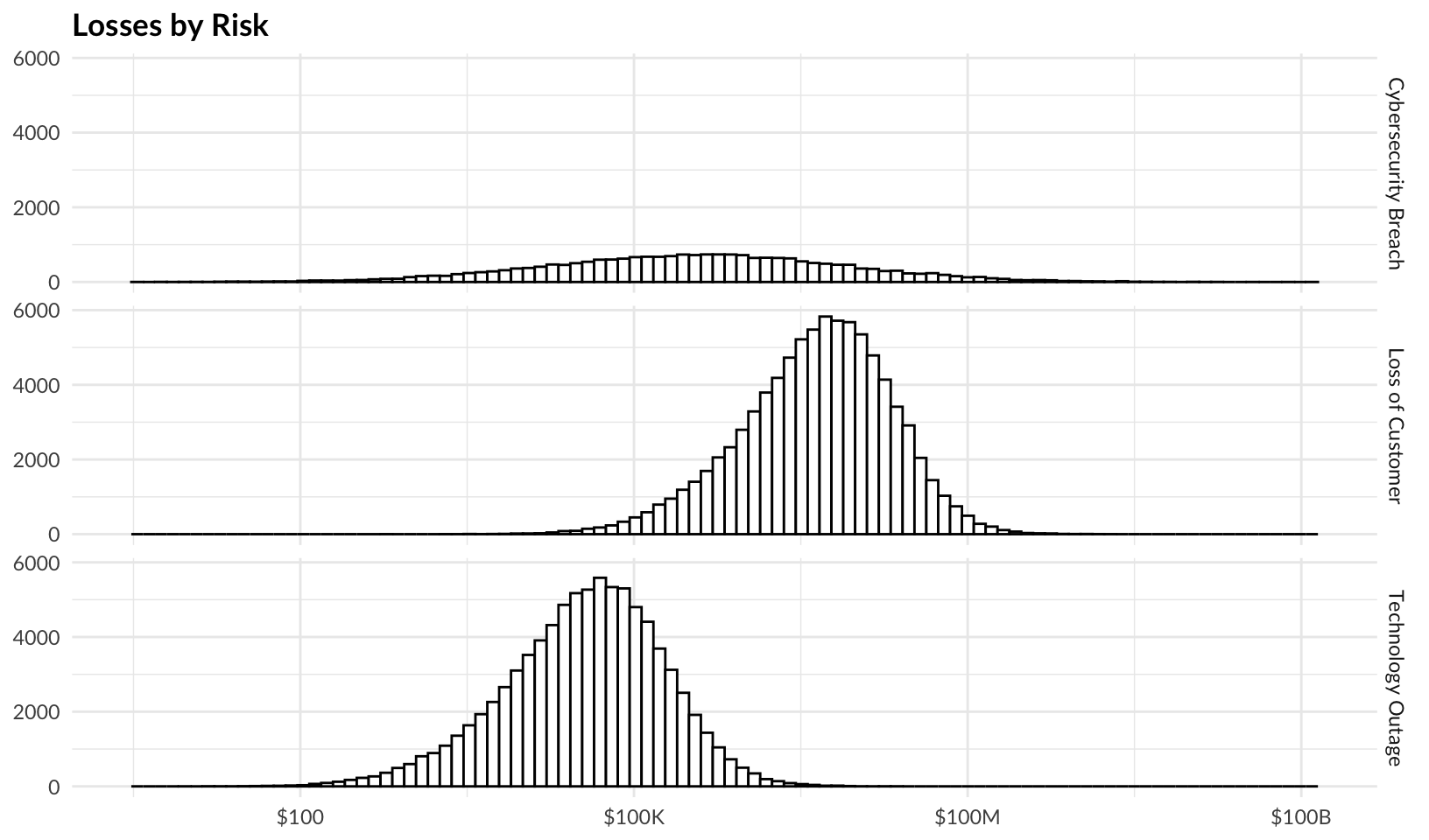
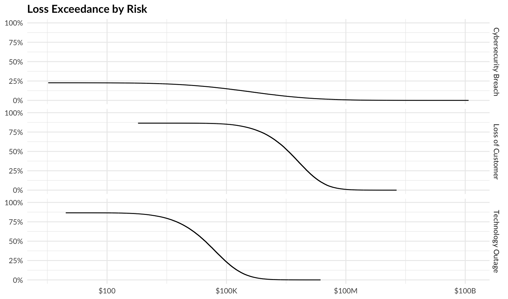
The Widget Management System (WMS) is over 30 years old and its architecture has not changed significantly since the original implementation. Over the years, the widget system has become an integral part of our services in managing widgets for our clients. In reviewing the system, three major risks were identified: First, the age of the technology prevents updating components of the system that no longer meet contemporary cybersecurity standards, which increases the likelihood of a breach. Second, the system is less reliable and experiences frequent outages, typically about 2 major outages per year, which results in lost revenue, contractual penalties, and overtime pay to recover from the incident. Third, limitations of the widget system have started to affect sales - we have recently lost a customer due to the functional obsolescence of the widget system, and expect to both lose more existing and prospective customers in the future due to increased competition in the widget management market.
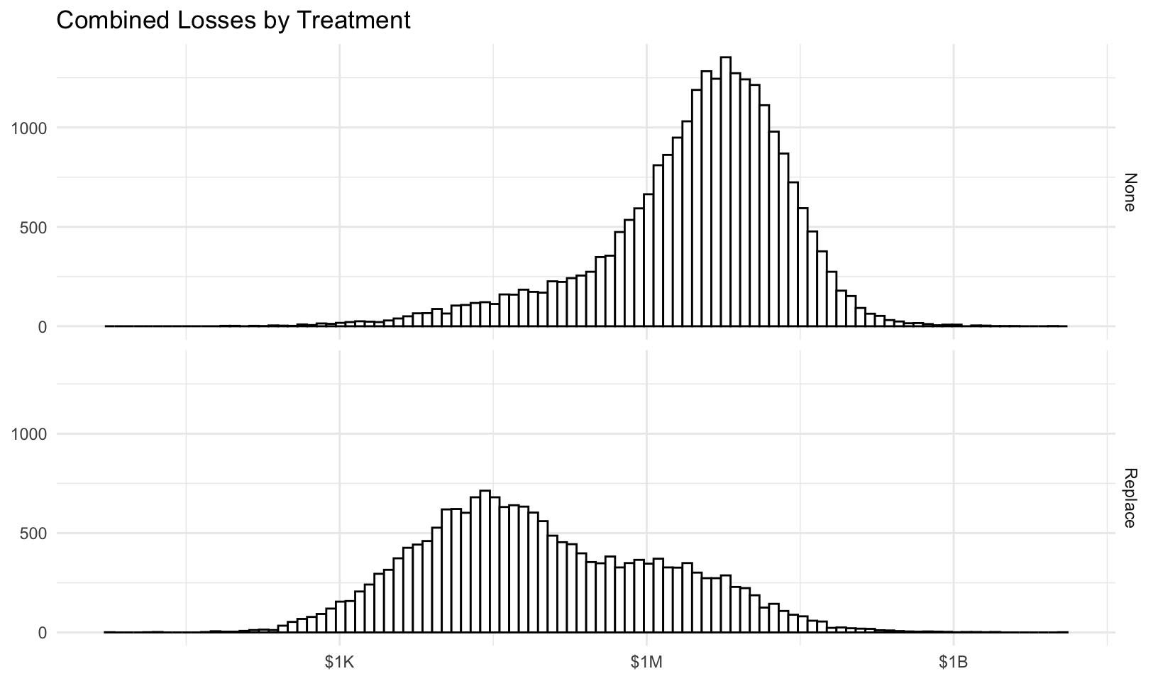
Experts were asked to consider two risk treatment scenarios:
None: The current system as it is today (baseline risk)
Replace: Complete replacement of the WMS with a modern, customer-centric solution
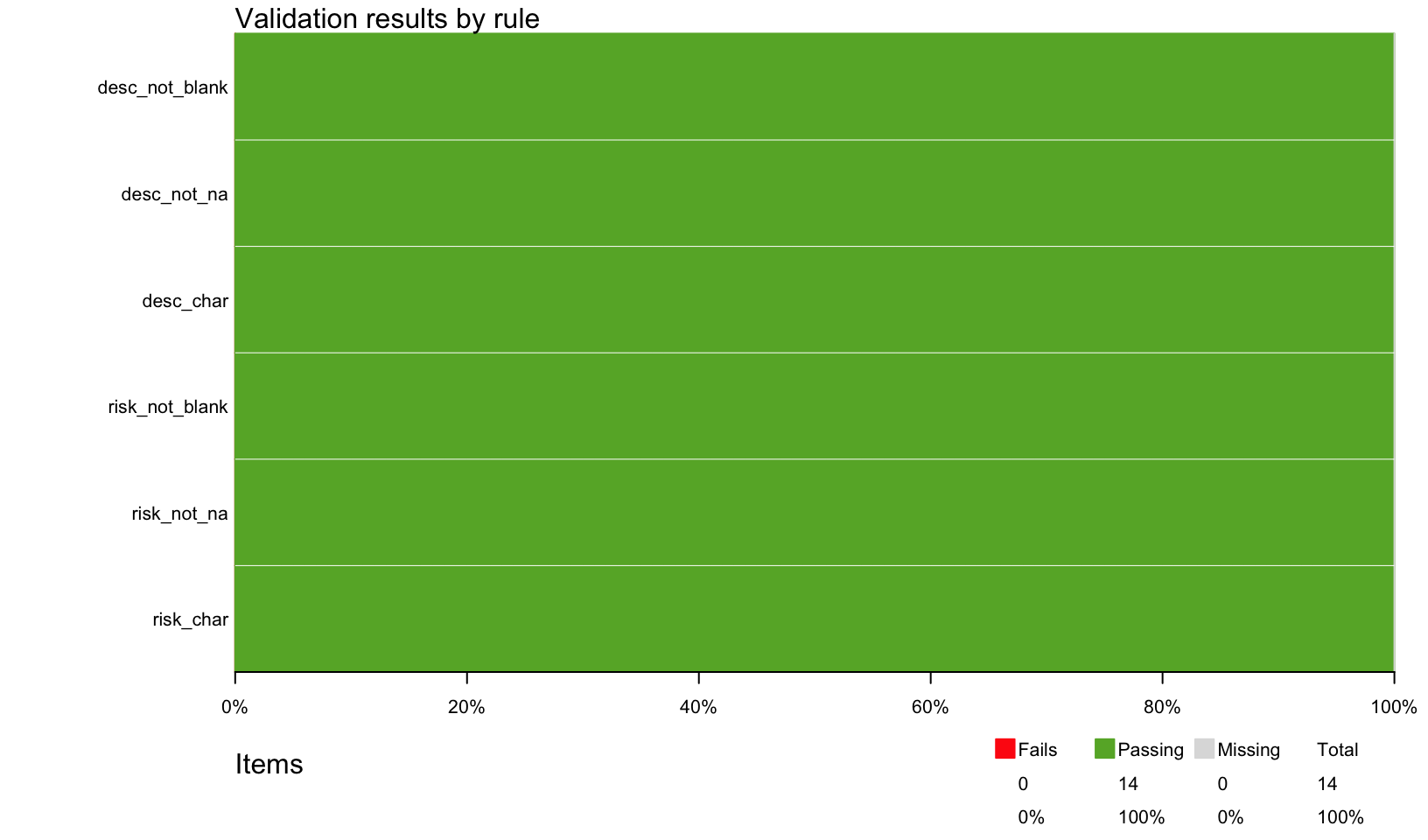
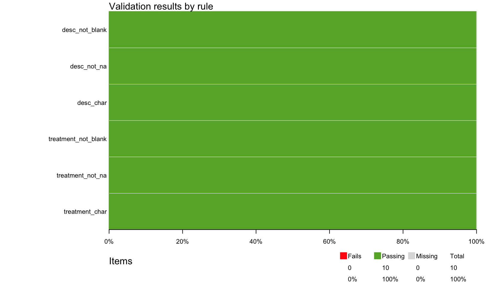
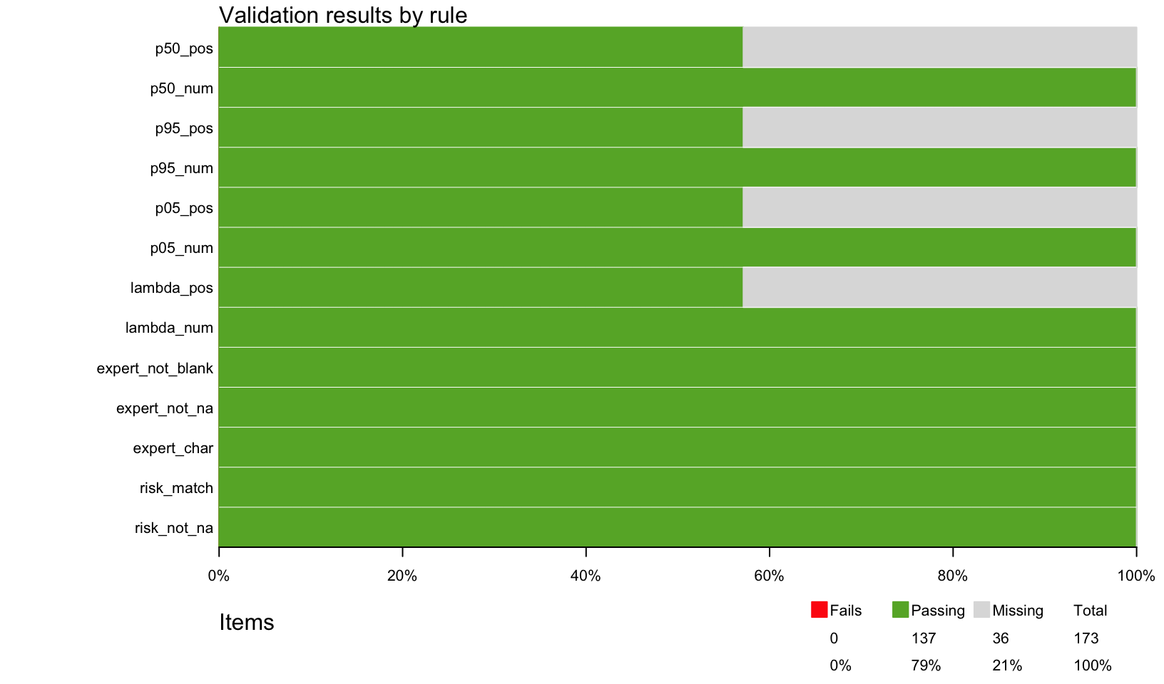
Import
Import and validate data from Excel.
The data was collected from 3 Technology SMEs, 3 Business SMEs, and one SME with experience in both. Experts were calibrated, informed by historical and industry data, and only gave estimates for areas in which they were confident in answering.
Forecast risk using Monte Carlo simulation. The average events, losses, ‘typical’ losses (geometric mean), and percentage of years with no losses for each risk and treatment are summarized below:
The consensus estimates for p05 and p95 result in the following parameters for log-normal loss magnitude. The p50 estimate is used to calculate the percentage difference from the actual median (mdiff), a measure of estimate accuracy:
year risk treatment events
Min. : 1 Length:150000 Length:150000 Min. : 0.0000
1st Qu.: 6251 Class :character Class :character 1st Qu.: 0.0000
Median :12500 Mode :character Mode :character Median : 0.0000
Mean :12500 Mean : 0.9581
3rd Qu.:18750 3rd Qu.: 2.0000
Max. :25000 Max. :10.0000
losses
Min. :0.000e+00
1st Qu.:0.000e+00
Median :0.000e+00
Mean :2.958e+06
3rd Qu.:1.364e+05
Max. :1.056e+10
Source Code
---title: "Widget System Risk Analysis Report"author: ""date: '2024-08-15'date-modified: '2025-08-18'categories: []order: 100format: html: code-fold: true code-tools: true code-link: trueoutput: html_notebook: theme: version: 5 preset: bootstrap pandoc_args: --shift-heading-level-by=1 toc: yes toc_float: collapsed: no smooth_scroll: no---Example [quantrr](https://jabenninghoff.github.io/quantrr/) risk analysis of the "Widget Management System" (WMS).```{r setup, message = FALSE, warning = FALSE}library(quantrr)library(readxl)library(janitor)library(validate)library(dplyr)library(formattable)library(purrr)library(ggplot2)library(plotly)# TODO: workaround for https://github.com/r-lib/lintr/issues/2790, update when# https://github.com/data-cleaning/validate/pull/197 is released (1.1.6+)is.nzchar <- nzchar # nolint: object_name_linter.# set the relative file path and name to importreport_file <-"data/widgetsys.xlsx"```# Environment StatementThe Widget Management System (WMS) is over 30 years old and its architecture has not changed significantly since the original implementation. Over the years, the widget system has become an integral part of our services in managing widgets for our clients. In reviewing the system, three major risks were identified: First, the age of the technology prevents updating components of the system that no longer meet contemporary cybersecurity standards, which increases the likelihood of a breach. Second, the system is less reliable and experiences frequent outages, typically about 2 major outages per year, which results in lost revenue, contractual penalties, and overtime pay to recover from the incident. Third, limitations of the widget system have started to affect sales - we have recently lost a customer due to the functional obsolescence of the widget system, and expect to both lose more existing and prospective customers in the future due to increased competition in the widget management market.Experts were asked to consider two risk treatment scenarios:- None: The current system as it is today (baseline risk)- Replace: Complete replacement of the WMS with a modern, customer-centric solution# ImportImport and validate data from Excel.The data was collected from 3 Technology SMEs, 3 Business SMEs, and one SME with experience in both. Experts were calibrated, informed by historical and industry data, and only gave estimates for areas in which they were confident in answering.```{r import}risks <-read_xlsx(report_file, sheet ="Risks") |>clean_names()validate_risks <-local({ validate_rules <-validator(risk_char =is.character(risk),risk_not_na =!is.na(risk),risk_not_blank =is.nzchar(risk, keep_na =TRUE),desc_char =is.character(description),desc_not_na =!is.na(description),desc_not_blank =is.nzchar(risk, keep_na =TRUE) )confront(risks, validate_rules)})check_validation(validate_risks, sheet ="Risks")treatments <-read_xlsx(report_file, sheet ="Treatments") |>clean_names()validate_treatments <-local({ validate_rules <-validator(treatment_char =is.character(treatment),treatment_not_na =!is.na(treatment),treatment_not_blank =is.nzchar(treatment, keep_na =TRUE),desc_char =is.character(description),desc_not_na =!is.na(description),desc_not_blank =is.nzchar(treatment, keep_na =TRUE) )confront(treatments, validate_rules)})check_validation(validate_treatments, sheet ="Treatments")estimates <-read_xlsx(report_file, sheet ="Estimates") |>clean_names() |>rename(lambda = frequency_per_yer, p05 = low_5_percent, p95 = high_95_percent, p50 = most_likely )validate_estimates <-local({ validate_rules <-validator(risk_not_na =!is.na(risk),risk_match = risk %in% risks$risk,expert_char =is.character(expert),expert_not_na =!is.na(expert),expert_not_blank =is.nzchar(expert, keep_na =TRUE),lambda_num =is.numeric(lambda),lambda_pos = lambda >0,p05_num =is.numeric(p05),p05_pos = p05 >0,p95_num =is.numeric(p95),p95_pos = p95 >0,p50_num =is.numeric(p50),p50_pos = p50 >0 )confront(estimates, validate_rules)})check_validation(validate_estimates, sheet ="Estimates")```# RisksRisk descriptions:```{r risks}formattable(risks, align ="l")```Treatment descriptions:```{r treatments}formattable(treatments, align ="l")```# ForecastForecast risk using Monte Carlo simulation. The average events, losses, 'typical' losses (geometricmean), and percentage of years with no losses for each risk and treatment are summarized below:```{r forecast}consensus <- estimates |>group_by(treatment, risk) |>summarize(across(lambda:p50, ~mean(.x, na.rm =TRUE)), .groups ="drop")consensus_params <- consensus |>mutate(as_tibble(lnorm_param(.data$p05, .data$p95, .data$p50)))forecast <- consensus_params |>select(c("risk", "lambda", "meanlog", "sdlog", "treatment")) |>pmap(calc_risk) |>list_rbind()forecast |>group_by(treatment, risk) |>mutate(no_losses = events ==0) |>summarize(avg_events =mean(events), avg_losses =mean(losses), typ_losses =gmean(losses),no_losses =mean(no_losses), .groups ="drop" ) |>mutate(across(avg_losses:typ_losses, ~currency(.x, digits =0L)),no_losses =percent(no_losses) ) |>formattable(align ="l")```# LossesBase losses (with no risk treatment) by risk:```{r risk_hist}forecast |>filter(tolower(treatment) =="none") |># remove zero losses to plot using log10 scalefilter(losses >0) |>ggplot(aes(losses)) +facet_grid(vars(risk)) +geom_histogram(color ="black", fill ="white", bins =100) +scale_x_log10(labels = scales::label_currency(scale_cut = scales::cut_short_scale())) +labs(x =NULL, y =NULL, title ="Base Losses by Risk") +theme_minimal()```Combined losses by treatment:```{r treatment_hist}forecast |>group_by(treatment, year) |>summarize(total_losses =sum(losses), .groups ="drop_last") |># remove zero losses to plot using log10 scalefilter(total_losses >0) |>ggplot(aes(total_losses)) +facet_grid(vars(treatment)) +geom_histogram(color ="black", fill ="white", bins =100) +scale_x_log10(labels = scales::label_currency(scale_cut = scales::cut_short_scale())) +labs(x =NULL, y =NULL, title ="Combined Losses by Treatment") +theme_minimal()```# Loss Exceedance CurvesPlot loss exceedance curves for all risks and combined risk, with risk treatments.## By RiskPlot loss exceedance curves for each risk:```{r risk_le}risk_le <- forecast |>group_by(risk, treatment) |>mutate(probability =1-percent_rank(losses)) |>filter(losses >0) |>ungroup() |>mutate(losses =currency(losses, digits =0), probability =percent(probability)) |>ggplot(aes(losses, probability, color = treatment)) +facet_grid(vars(risk)) +geom_line() +scale_y_continuous(labels = scales::label_percent(), limits =c(0, 1)) +scale_x_log10(labels = scales::label_currency(scale_cut = scales::cut_short_scale())) +labs(x =NULL, y =NULL, color ="Treatment", title ="Loss Exceedance by Risk") +scale_color_viridis_d() +theme_minimal()risk_le```Interactive plot:```{r risk_le_plotly}ggplotly(risk_le +guides(color ="none"))```## Combined RiskPlot loss exceedance curve for combined risk:```{r combined_le}combined_le <- forecast |>group_by(treatment, year) |>summarize(total_losses =sum(losses), .groups ="drop_last") |>mutate(probability =1-percent_rank(total_losses)) |>filter(total_losses >0) |>ungroup() |>mutate(total_losses =currency(total_losses, digits =0), probability =percent(probability)) |>ggplot(aes(total_losses, probability, color = treatment)) +geom_line() +scale_y_continuous(labels = scales::label_percent(), limits =c(0, 1)) +scale_x_log10(labels = scales::label_currency(scale_cut = scales::cut_short_scale())) +labs(x =NULL, y =NULL, color ="Treatment", title ="Combined Loss Exceedance") +scale_color_viridis_d() +theme_minimal()combined_le```Interactive plot:```{r combined_le_plotly}ggplotly(combined_le +guides(color ="none"))```# AppendixAdditional details on the risk quantification analysis.## ValidationData validation results for Risks tab:```{r validate_risks}plot(validate_risks)```Data validation results for Treatments tab:```{r validate_treatments}plot(validate_treatments)```Data validation results for Estimates tab:```{r validate_estimates}plot(validate_estimates)```## EstimatesAll risk estimates:```{r estimates}estimates |>mutate(across(p05:p50, ~currency(.x, digits =0L))) |>formattable(align ="l")```## Consensus EstimateUsing a simple average of all experts that provided an estimate (not blank/NA), this gives us aconsensus estimate for the three risks of:```{r consensus}consensus |>mutate(across(p05:p50, ~currency(.x, digits =0L))) |>formattable(align ="l")```The consensus estimates for p05 and p95 result in the following parameters for log-normal lossmagnitude. The p50 estimate is used to calculate the percentage difference from the actual median(`mdiff`), a measure of estimate accuracy:```{r consensus_params}consensus_params |>mutate(across(p05:p50, ~currency(.x, digits =0L)), mdiff =percent(mdiff)) |>formattable(align ="l")```## Forecast SummaryA `summary()` of the forecast results.```{r summary}summary(forecast)```