jbplot ggplot2 style

library(jbplot)
library(ggplot2)
library(showtext)

font_add_google("Lato", "Lato")

jbplot includes functions to change the style of ggplot2 plots. The included theme, quo, can be added to individual plots using theme_quo().

Quo Theme

The quo theme applied to the venerable mtcars dataset. Example adapted from ggplot2::theme_minimal():

p1 <- ggplot(mtcars, aes(x = wt, y = mpg, color = factor(cyl))) +
  geom_point() +
  labs(
    title = "Fuel economy declines as weight increases",
    subtitle = "(1973-74)",
    caption = "Data from the 1974 Motor Trend US magazine.",
    tag = "Figure 1",
    x = "Weight (1000 lbs)",
    y = "Fuel economy (mpg)",
    color = "Gears"
  )

p1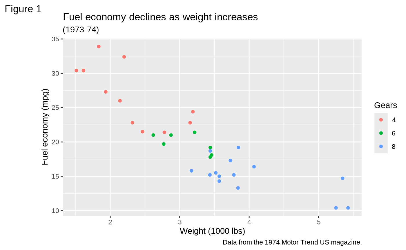

p1 + theme_quo()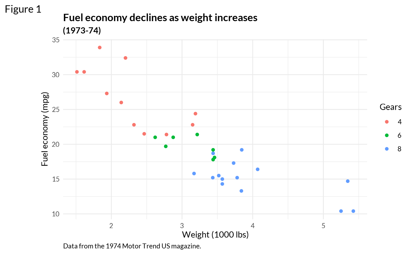

The viridis color scheme can be added manually using ggplot2::scale_color_viridis_d():

p1 +
  theme_quo() +
  scale_color_viridis_d()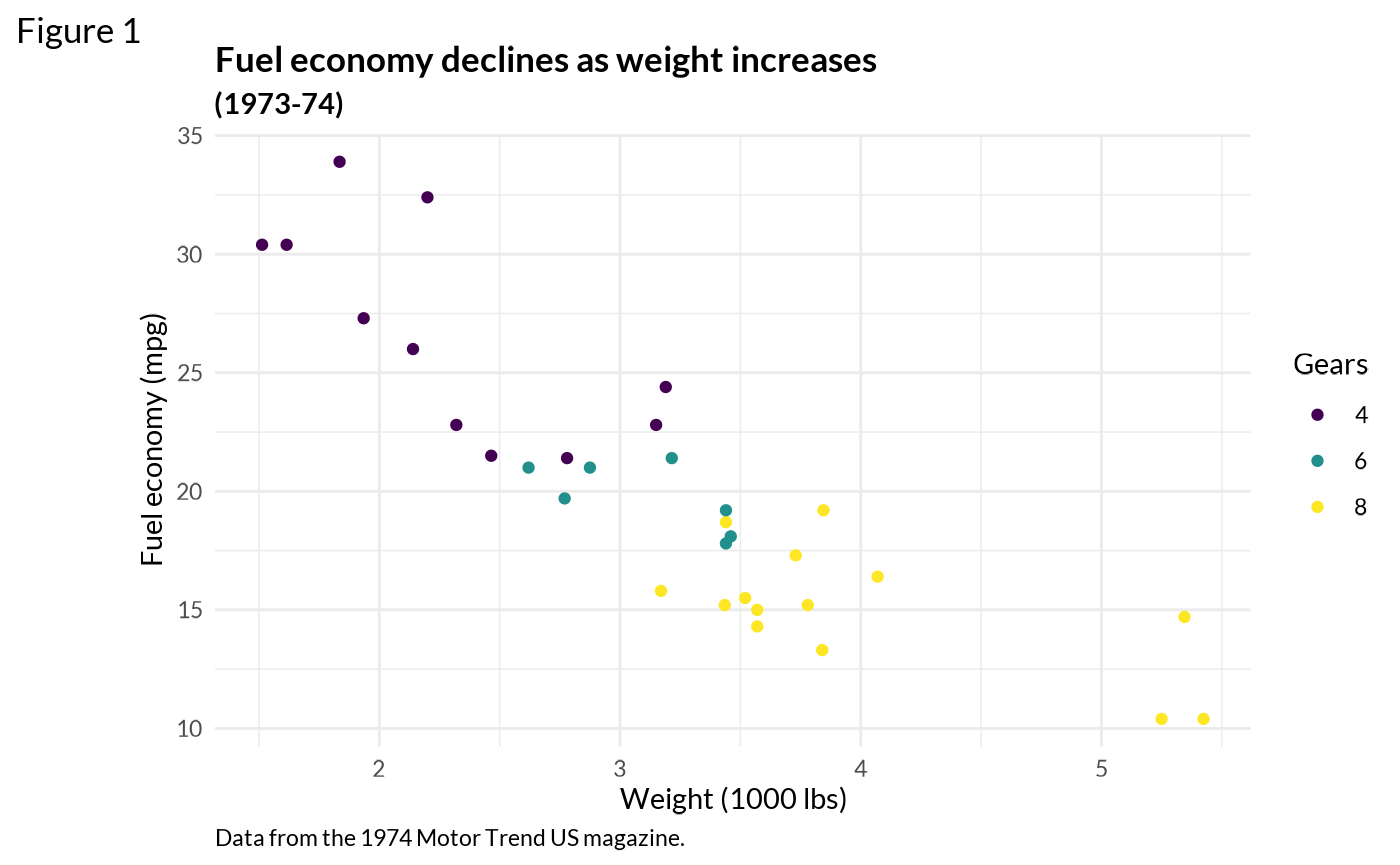

Viridis Quo

Quo is designed to be paired with the viridis color scale, added by calling one of the continuous (c) or discrete (d) viridis color scales:

• ggplot2::scale_color_viridis_c()
• ggplot2::scale_fill_viridis_c()
• ggplot2::scale_color_viridis_d()
• ggplot2::scale_fill_viridis_d()

Sample plots using the default theme and color scales:

txsamp <- subset(txhousing, city %in% c("Houston", "Fort Worth", "San Antonio", "Dallas", "Austin"))

(d <- ggplot(data = txsamp, aes(x = sales, y = median)) +
  geom_point(aes(colour = city)))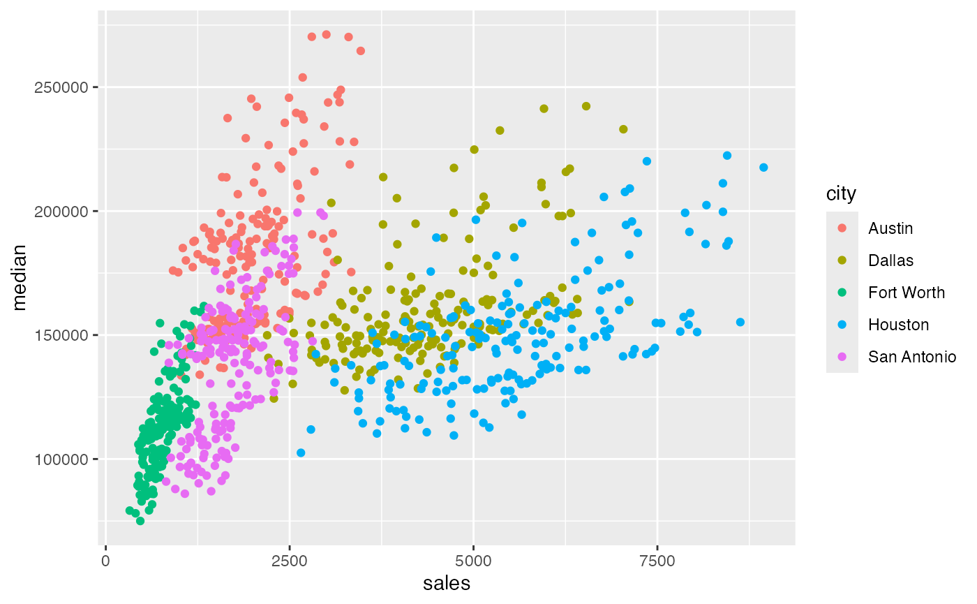

(p <- ggplot(txsamp, aes(x = median, fill = city)) +
  geom_histogram(position = "dodge", binwidth = 15000))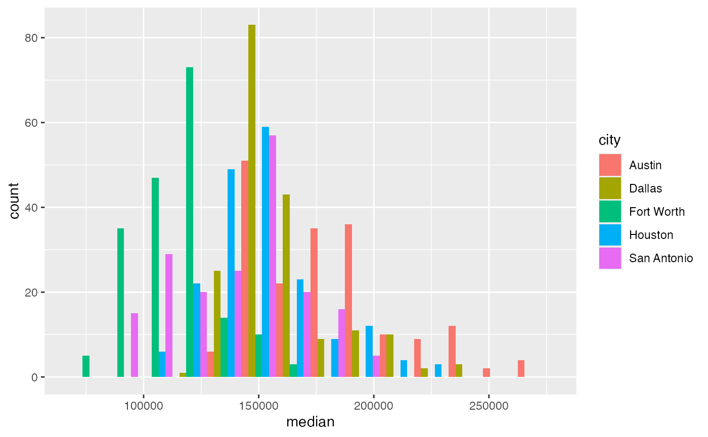

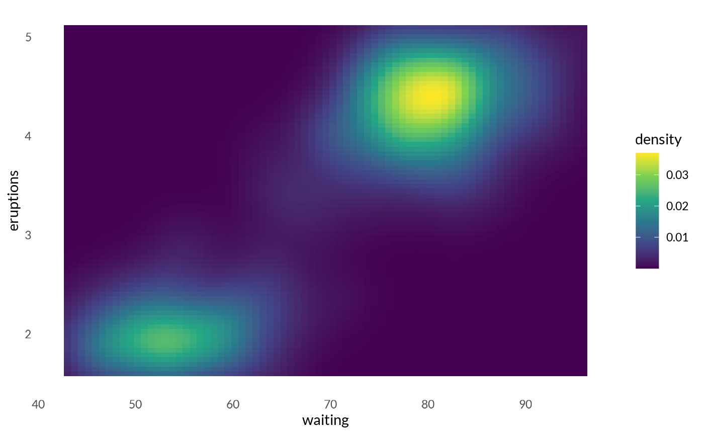
(v <- ggplot(faithfuld) +
  geom_raster(aes(waiting, eruptions, fill = density)))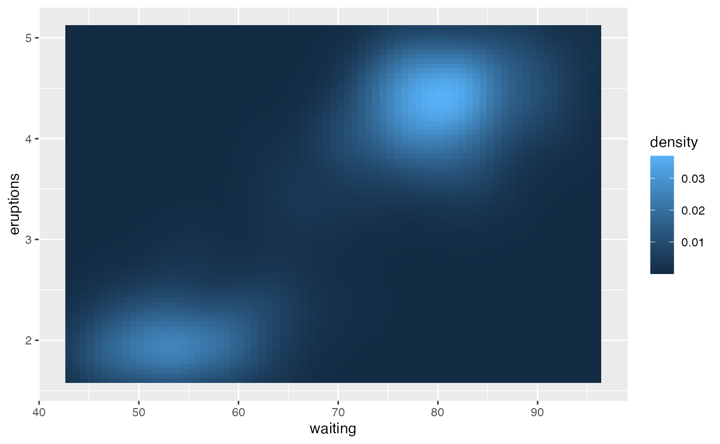

The same plots after applying viridis and quo:

d + scale_color_viridis_d() + theme_quo()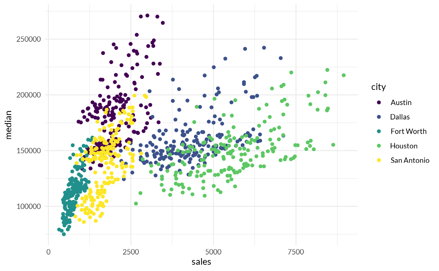

p + scale_fill_viridis_d() + theme_quo()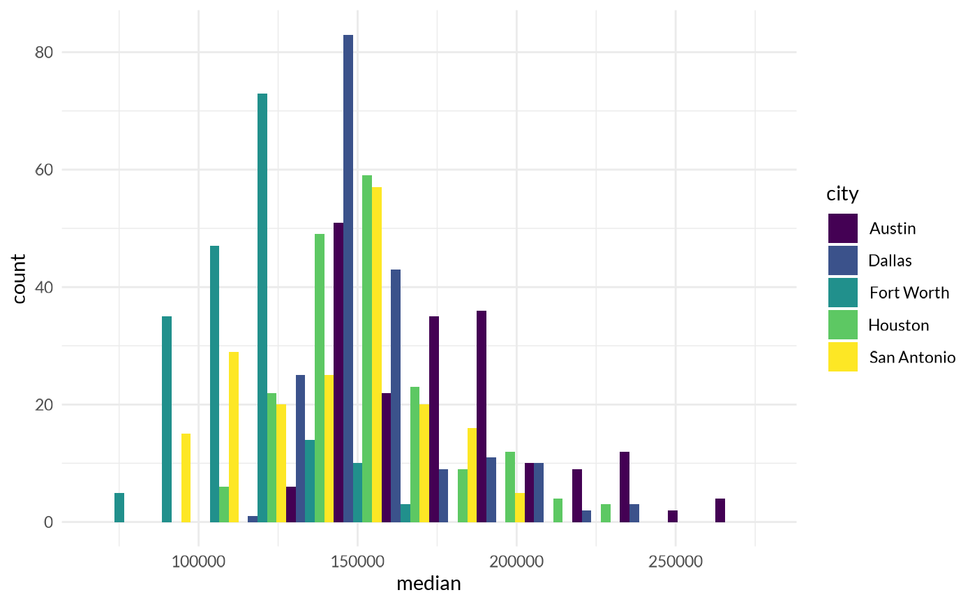

v + scale_fill_viridis_c() + theme_quo()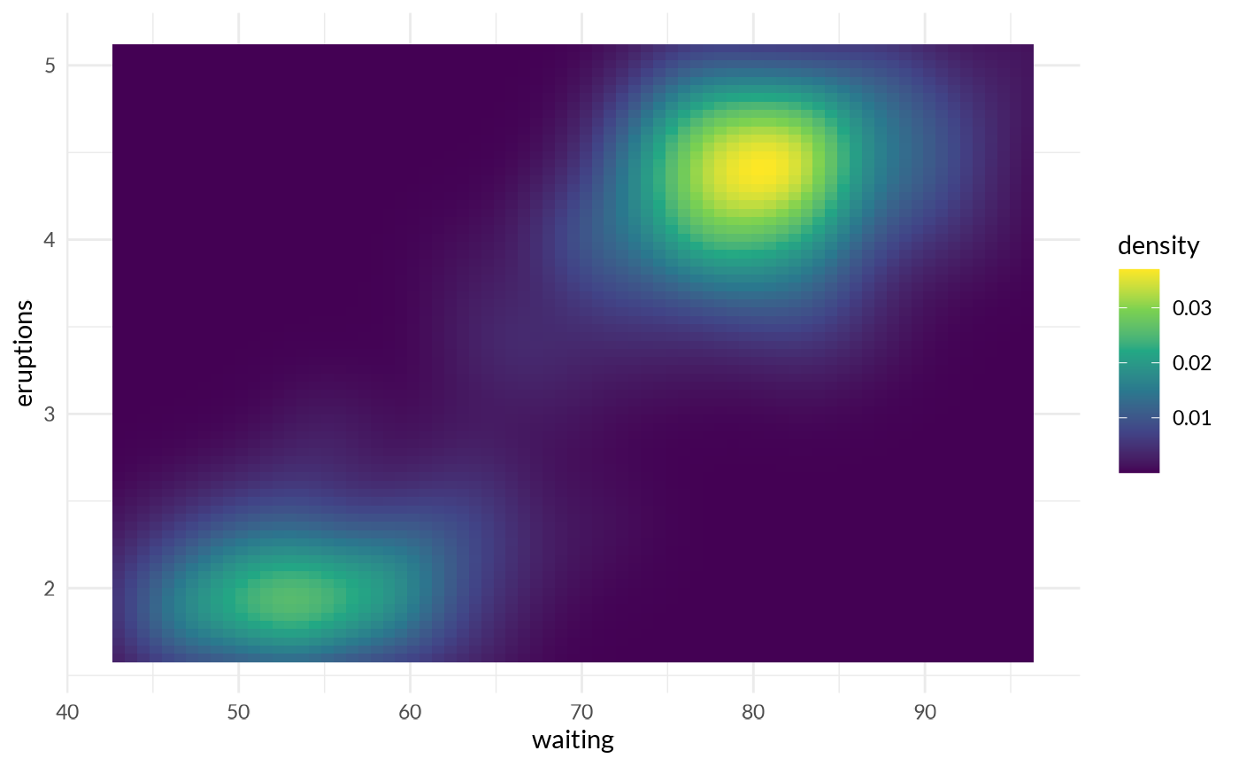

Grid lines

Grid lines can be selectively disabled using theme_quo():

d + scale_color_viridis_d() + theme_quo(minor = FALSE)

p + scale_fill_viridis_d() + theme_quo(x = FALSE)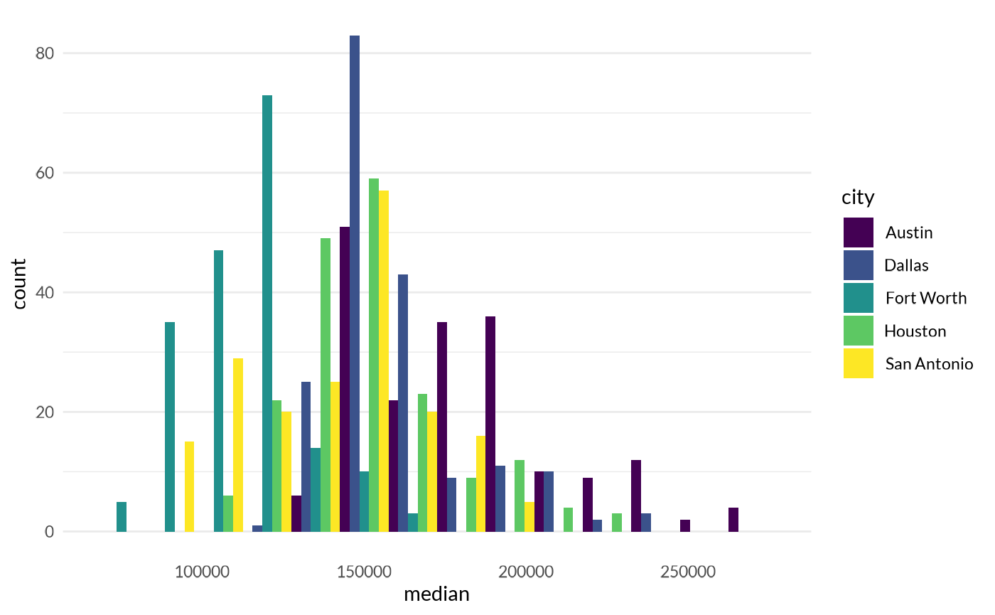

v + scale_fill_viridis_c() + theme_quo(major = FALSE, minor = FALSE)